1 Empirical Applications of Linear & Nonlinear Regressions
This chapter introduces the basics in linear and nonlinear regression models and shows how to perform regression analysis in R.
The following packages are needed for reproducing the code presented in this chapter:
AER- accompanies the Book Applied Econometrics with R by C. Kleiber and Zeileis (2008) and provides useful functions and data sets.MASS- a collection of functions for applied statistics.stargazer- used for creating well-formatted regression and summary statistics tables (Hlavac 2022)
1.1 Data Set Description
The California School data set (CASchools) is included in the R package “AER”. This dataset contains information on various characteristics of schools in California, such as test scores, teacher salaries, and student demographics. It’s commonly used in econometrics and statistical analysis to explore relationships between these variables and to illustrate various modeling techniques.
   district            school                  county      grades
 Length:420         Length:420         Sonoma     : 29   KK-06: 61
 Class :character   Class :character   Kern       : 27   KK-08:359
 Mode  :character   Mode  :character   Los Angeles: 27
                                       Tulare     : 24
                                       San Diego  : 21
                                       Santa Clara: 20
                                       (Other)    :272
    students          teachers          calworks          lunch
 Min.   :   81.0   Min.   :   4.85   Min.   : 0.000   Min.   :  0.00
 1st Qu.:  379.0   1st Qu.:  19.66   1st Qu.: 4.395   1st Qu.: 23.28
 Median :  950.5   Median :  48.56   Median :10.520   Median : 41.75
 Mean   : 2628.8   Mean   : 129.07   Mean   :13.246   Mean   : 44.71
 3rd Qu.: 3008.0   3rd Qu.: 146.35   3rd Qu.:18.981   3rd Qu.: 66.86
 Max.   :27176.0   Max.   :1429.00   Max.   :78.994   Max.   :100.00

    computer       expenditure       income          english
 Min.   :   0.0   Min.   :3926   Min.   : 5.335   Min.   : 0.000
 1st Qu.:  46.0   1st Qu.:4906   1st Qu.:10.639   1st Qu.: 1.941
 Median : 117.5   Median :5215   Median :13.728   Median : 8.778
 Mean   : 303.4   Mean   :5312   Mean   :15.317   Mean   :15.768
 3rd Qu.: 375.2   3rd Qu.:5601   3rd Qu.:17.629   3rd Qu.:22.970
 Max.   :3324.0   Max.   :7712   Max.   :55.328   Max.   :85.540

      read            math
 Min.   :604.5   Min.   :605.4
 1st Qu.:640.4   1st Qu.:639.4
 Median :655.8   Median :652.5
 Mean   :655.0   Mean   :653.3
 3rd Qu.:668.7   3rd Qu.:665.9
 Max.   :704.0   Max.   :709.5
Upon examination we find that the dataset contains mostly numeric variables, but it lacks two important ones we’re interested in: average test scores and student-teacher ratios. However, we can calculate them using the available data. To find the student-teacher ratio, we divide the total number of students by the number of teachers. For the average test score, we just need to average the math and reading scores. In the next code chunk, we’ll demonstrate how to create these variables as vectors and add them to the CASchools dataset.
# compute student-teacher ratio and append it to CASchools
CASchools$STR <- CASchools$students/CASchools$teachers

# compute test score and append it to CASchools
CASchools$score <- (CASchools$read + CASchools$math)/2
If we ran summary(CASchools) again we would find the two variables of interest as additional variables named STR and score.
2 Linear Regression
Let’s suppose we were interested in the following regression model
TestScore = \beta_0 + \beta_1 \, STR + \beta_2 \, english + u
In this regression, we aim to explore how test scores (TestScore) are influenced by student-teacher ratio (STR) and the percentage of English learners (english). The variable english indicates the proportion of students who may require additional support or resources to improve their English language skills within each school.
We would run this model in R using the lm() function and explore the regression estimates with coeftest().
# run the model
model <- lm(score ~ STR + english, data = CASchools)
# report estimates
coeftest(model, vcov. = vcovHC, type = "HC1")
t test of coefficients:

              Estimate Std. Error  t value Pr(>|t|)
(Intercept) 686.032245   8.728225  78.5993  < 2e-16 ***
STR          -1.101296   0.432847  -2.5443  0.01131 *
english      -0.649777   0.031032 -20.9391  < 2e-16 ***
---
Signif. codes:  0 '***' 0.001 '**' 0.01 '*' 0.05 '.' 0.1 ' ' 1
2.0.1 Hypothesis Tests and Confidence Intervals for a Single Coefficient
The coeftest() function in R, along with suitable options such as vcov. = vcovHC for robust standard errors, automatically includes statistics such as standard errors, t-statistics, and p-values, which is exactly what we need to test hypotheses about single coefficients (\beta_j) in regression models.
We could also manually check these values calculating the t-statistics or p-values using the provided output above and using R as a calculator. For example, using the definition of the p-value for a two-sided test, we can confirm the p-value for a test of the hypothesis that the coefficient \beta_1, which represents the coefficient onSTR, is approximately 0.01
# compute two-sided p-value
2 * (1 - pt(abs(coeftest(model, vcov. = vcovHC, type = "HC1")[2, 3]),
            df = model$df.residual))
[1] 0.01130921We can also compute confidence intervals for individual coefficients in the multiple regression model by using the function confint(). This function computes confidence intervals at the 95% level by default.
# compute confidence intervals for all coefficients in the model
confint(model)
2.5 % 97.5 %
(Intercept) 671.4640580 700.6004311
STR -1.8487969 -0.3537944
english -0.7271113 -0.5724424To obtain confidence intervals at a different level, say 90%, we set the argument level in our call of confint() accordingly.
confint(model, level = 0.9) 5 % 95 %
(Intercept) 673.8145793 698.2499098
STR -1.7281904 -0.4744009
english -0.7146336 -0.5849200A limitation of using confint() is its failure to incorporate robust standard errors when computing confidence intervals. To address this, you can manually generate large-sample confidence intervals that consider robust standard errors with the following method.
# compute robust standard errors
rob_se <- diag(vcovHC(model, type = "HC1"))^0.5

# compute robust 95% confidence intervals
rbind("lower" = coef(model) - qnorm(0.975) * rob_se,
      "upper" = coef(model) + qnorm(0.975) * rob_se)
(Intercept) STR english
lower 668.9252 -1.9496606 -0.7105980
upper 703.1393 -0.2529307 -0.5889557# compute robust 90% confidence intervals
rbind("lower" = coef(model) - qnorm(0.95) * rob_se,
"upper" = coef(model) + qnorm(0.95) * rob_se) (Intercept) STR english
lower 671.6756 -1.8132659 -0.7008195
upper 700.3889 -0.3893254 -0.5987341The output above shows that zero is not an element of the confidence interval for the coefficient on STR, so we can reject the null hypothesis at significance levels of 5\% and 10\% (Note that rejection at the 5\% level implies rejection at the 10\% level anyway). We can bring this conclusion further via the p-value for STR: 0.00398<0.01, which indicates that this coefficient estimate is significant at the 1\% level.
2.0.2 Joint Hypothesis Testing
Let’s suppose now that we are interested in investigating the average effect on test scores of reducing the student-teacher ratio when the expenditures per pupil and the percentage of english learning pupils are held constant. Let us augment our model by an additional regressor expenditure, that is a measure for the total expenditure per pupil in the district. For this model, we will include expenditure as measured in thousands of dollars. Our new model would be
TestScore = \beta_0 + \beta_1 \, STR + \beta_2 \, english + \beta_3 \, expenditure + u
Let us now estimate the model:
# scale expenditure to thousands of dollars
CASchools$expenditure <- CASchools$expenditure/1000

# estimate the model
model <- lm(score ~ STR + english + expenditure, data = CASchools)
coeftest(model, vcov. = vcovHC, type = "HC1")
t test of coefficients:

              Estimate Std. Error  t value Pr(>|t|)
(Intercept) 649.577947  15.458344  42.0212  < 2e-16 ***
STR          -0.286399   0.482073  -0.5941  0.55277
english      -0.656023   0.031784 -20.6398  < 2e-16 ***
expenditure   3.867901   1.580722   2.4469  0.01482 *
---
Signif. codes:  0 '***' 0.001 '**' 0.01 '*' 0.05 '.' 0.1 ' ' 1
The estimated impact of a one-unit change in the student-teacher ratio on test scores, while holding expenditure and the proportion of English learners constant, is -0.29. It is much smaller than the estimated coefficient in our initial model where we didn’t include expenditure. Additionally, this coefficient of STR is no longer statistically significant, even at a 10\% significance level, as indicated by a p-value of 0.55. This lack of significance for \beta_1 may stem from a larger standard error resulting from the inclusion of expenditure in the model, leading to less precise estimation of the coefficient on STR. This scenario highlights the challenge of dealing with strongly correlated predictors, known as imperfect multicollinearity. The correlation between STR and expenditure can be determined using the cor() function.
# compute the sample correlation between 'STR' and 'expenditure'
cor(CASchools$STR, CASchools$expenditure)
[1] -0.6199822This indicates a moderately strong negative correlation between the two variables.
The estimated model is
\widehat{TestScore} = \underset{(15.21)}{649.58} \,- \underset{(0.48)}{0.29} \, STR - \underset{(0.04)}{0.66} \, english + \underset{(1.41)}{3.87} \, expenditure Could we reject the hypothesis that both the STR coefficient and the expenditure coefficient are zero? To answer this, we need to conduct joint hypothesis tests, which involve placing restrictions on multiple regression coefficients. This differs from individual t-tests, where restrictions are applied to a single coefficient.
To test whether both coefficients are zero, we will conduct an F-test. To do this in R, we can use the function linearHypothesis() contained in the package car.
# execute the function on the model object and provide both linear restrictions
# to be tested as strings
linearHypothesis(model, c("STR=0", "expenditure=0"))
Linear hypothesis test
Hypothesis:
STR = 0
expenditure = 0
Model 1: restricted model
Model 2: score ~ STR + english + expenditure
Res.Df RSS Df Sum of Sq F Pr(>F)
1 418 89000
2 416 85700 2 3300.3 8.0101 0.000386 ***
---
Signif. codes: 0 '***' 0.001 '**' 0.01 '*' 0.05 '.' 0.1 ' ' 1The output reveals that the F-statistic for this joint hypothesis test is 8.01 and the corresponding p-value is about 0.0004. We can therefore reject the null hypothesis that both coefficients are zero at the 0.1\% level of significance.
A heteroskedasticity-robust version of this F-test (which leads to the same conclusion) can be conducted as follows:
# heteroskedasticity-robust F-test
linearHypothesis(model, c("STR=0", "expenditure=0"), white.adjust = "hc1")
Linear hypothesis test
Hypothesis:
STR = 0
expenditure = 0
Model 1: restricted model
Model 2: score ~ STR + english + expenditure
Note: Coefficient covariance matrix supplied.
Res.Df Df F Pr(>F)
1 418
2 416 2 5.4337 0.004682 **
---
Signif. codes: 0 '***' 0.001 '**' 0.01 '*' 0.05 '.' 0.1 ' ' 1The standard output of a model summary in R also reports an F-statistic and the corresponding p-value. This F-test examines whether all of the population coefficients in the model except for the intercept are zero, so the hypotheses would be H_0: \beta_1=0, \beta_2=0, \beta_3=0 vs. H_1: \beta_j \neq 0 for at least one j=1,2,3.
We now check whether the F-statistic belonging to the p-value listed in the model’s summary matches with the result reported by linearHypothesis()
# execute the function on the model object and provide the restrictions
# to be tested as a character vector
linearHypothesis(model, c("STR=0", "english=0", "expenditure=0"))
Linear hypothesis test
Hypothesis:
STR = 0
english = 0
expenditure = 0
Model 1: restricted model
Model 2: score ~ STR + english + expenditure
Res.Df RSS Df Sum of Sq F Pr(>F)
1 419 152110
2 416 85700 3 66410 107.45 < 2.2e-16 ***
---
Signif. codes: 0 '***' 0.001 '**' 0.01 '*' 0.05 '.' 0.1 ' ' 1# Access the overall F-statistic from the model's summary
summary(model)$fstatistic value numdf dendf
107.4547 3.0000 416.0000 Both results match. The F-test rejects the null hypothesis that the model has no power in explaining test scores. It is nevertheless important to note that the F-statistic reported by summary is not robust to heteroskedasticity.
2.1 Multiple Regression
In order to reduce the risk of omitted variable bias, it is essential to include control variables in regression models. In our case, we are interested in estimating the causal effect of a change in the student-teacher ratio on test scores. We will now see an example of how to use multiple regression in order to alleviate omitted variable bias and how to report these results using R.
By including english as control variable, we aimed to control for unobservable student characteristics which correlate with the student-teacher ratio and are assumed to have an impact on test score. But there are other interesting variables to observe:
lunch: the share of students that qualify for a subsidized or even a free lunch at school.calworks: the percentage of students that qualify for the CalWorks income assistance program.
Students eligible for CalWorks live in families with a total income below the threshold for the subsidized lunch program, so both variables are indicators for the share of economically disadvantaged children. We suspect both indicators are highly correlated.
# estimate the correlation between 'calworks' and 'lunch'
cor(CASchools$calworks, CASchools$lunch)
[1] 0.7394218If they are highly correlated as we just confirmed, there is no standard way to proceed when deciding which variable to use. In any case it may not be a good idea to use both variables as regressors in view of collinearity. Let’s first explore further these control variables and how they correlate with the dependent variable by plotting them against test scores. When computing simultaneously several plots, we may use layout() to divide the plotting area and the matrix m to specify the location of the plots (see ?layout).
# set up arrangement of plots
m <- rbind(c(1, 2), c(3, 0))
graphics::layout(mat = m)

# scatterplots
plot(score ~ english,
     data = CASchools,
     col = "steelblue",
     pch = 20,
     xlim = c(0, 100),
     cex.main = 0.7,
     xlab="English",
     ylab="Score",
     main = "Percentage of English language learners")

plot(score ~ lunch,
     data = CASchools,
     col = "steelblue",
     pch = 20,
     cex.main = 0.7,
     xlab="Lunch",
     ylab="Score",
     main = "Percentage qualifying for reduced price lunch")

plot(score ~ calworks,
     data = CASchools,
     col = "steelblue",
     pch = 20,
     xlim = c(0, 100),
     cex.main = 0.7,
     xlab="CalWorks",
     ylab="Score",
     main = "Percentage qualifying for income assistance")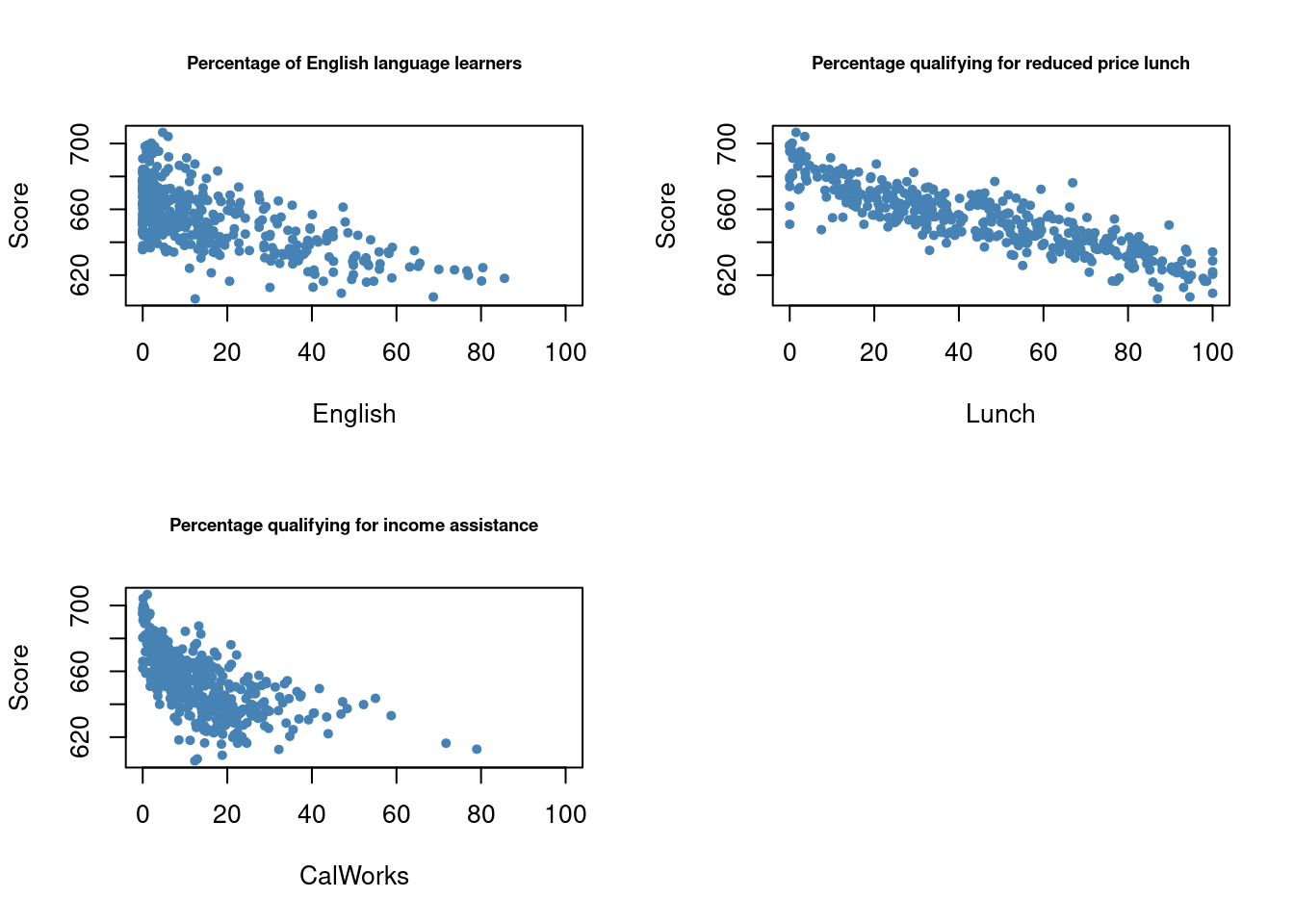
We observe negative relationships. Let’s check the correlation coefficients.
# estimate correlation between student characteristics and test scores
cor(CASchools$score, CASchools$english)
[1] -0.6441238cor(CASchools$score, CASchools$lunch)[1] -0.868772cor(CASchools$score, CASchools$calworks)[1] -0.6268533We shall consider five different model equations:
\begin{align} \text{TestScore} &= \beta_0 + \beta_1 \, \text{STR} + u, \\ \text{TestScore} &= \beta_0 + \beta_1 \, \text{STR} + \beta_2 \, \text{english} + u, \\ \text{TestScore} &= \beta_0 + \beta_1 \, \text{STR} + \beta_2 \, \text{english} + \beta_3 \, \text{lunch} + u, \\ \text{TestScore} &= \beta_0 + \beta_1 \, \text{STR} + \beta_2 \, \text{english} + \beta_4 \, \text{calworks} + u, \\ \text{TestScore} &= \beta_0 + \beta_1 \, \text{STR} + \beta_2 \, \text{english} + \beta_3 \, \text{lunch} + \beta_4 \, \text{calworks} + u. \end{align}
The best way to report regression results is in a table. The stargazer package is very convenient for this purpose. It provides a function that generates professionally looking HTML and LaTeX tables that satisfy scientific standards. One simply has to provide one or multiple object(s) of class lm. The rest is done by the function stargazer().
# load the stargazer library
library(stargazer)

# estimate different model specifications
spec1 <- lm(score ~ STR, data = CASchools)
spec2 <- lm(score ~ STR + english, data = CASchools)
spec3 <- lm(score ~ STR + english + lunch, data = CASchools)
spec4 <- lm(score ~ STR + english + calworks, data = CASchools)
spec5 <- lm(score ~ STR + english + lunch + calworks, data = CASchools)

# gather robust standard errors in a list
rob_se <- list(sqrt(diag(vcovHC(spec1, type = "HC1"))),
               sqrt(diag(vcovHC(spec2, type = "HC1"))),
               sqrt(diag(vcovHC(spec3, type = "HC1"))),
               sqrt(diag(vcovHC(spec4, type = "HC1"))),
               sqrt(diag(vcovHC(spec5, type = "HC1"))))

# generate a LaTeX table using stargazer
stargazer(spec1, spec2, spec3, spec4, spec5,
          se = rob_se,
          type = "text",
          digits = 3,
          header = F,
          column.labels = c("(I)", "(II)", "(III)", "(IV)", "(V)"))
===============================================================================================================================================
                                                                        Dependent variable:
                    ---------------------------------------------------------------------------------------------------------------------------
                                                                               score
                              (I)                     (II)                    (III)                     (IV)                     (V)
                              (1)                     (2)                      (3)                      (4)                      (5)
-----------------------------------------------------------------------------------------------------------------------------------------------
STR                        -2.280***                -1.101**                -0.998***                -1.308***                -1.014***
                            (0.519)                 (0.433)                  (0.270)                  (0.339)                  (0.269)

english                                            -0.650***                -0.122***                -0.488***                -0.130***
                                                    (0.031)                  (0.033)                  (0.030)                  (0.036)

lunch                                                                       -0.547***                                         -0.529***
                                                                             (0.024)                                           (0.038)

calworks                                                                                             -0.790***                  -0.048
                                                                                                      (0.068)                  (0.059)

Constant                  698.933***               686.032***               700.150***               697.999***               700.392***
                           (10.364)                 (8.728)                  (5.568)                  (6.920)                  (5.537)

-----------------------------------------------------------------------------------------------------------------------------------------------
Observations                  420                     420                      420                      420                      420
R2                           0.051                   0.426                    0.775                    0.629                    0.775
Adjusted R2                  0.049                   0.424                    0.773                    0.626                    0.773
Residual Std. Error    18.581 (df = 418)       14.464 (df = 417)         9.080 (df = 416)        11.654 (df = 416)         9.084 (df = 415)
F Statistic         22.575*** (df = 1; 418) 155.014*** (df = 2; 417) 476.306*** (df = 3; 416) 234.638*** (df = 3; 416) 357.054*** (df = 4; 415)
===============================================================================================================================================
Note:                                                                                                               *p<0.1; **p<0.05; ***p<0.01
Each column in this table contains most of the information provided also by coeftest() and summary() for each of the models under consideration. Each of the coefficient estimates includes its standard error in parenthesis and one, two or three asterisks representing their significance levels. Although t-statistics are not reported, one may compute them manually simply by dividing a coefficient estimate by the corresponding standard error. At the bottom of the table summary statistics for each model and a legend are reported.
From the model comparison we observe that including control variables approximately cuts the coefficient on STR in half. Additionally, the estimation seems to remain unaffected by the specific set of control variables employed. Thus, the inference drawn is that, under all other conditions held constant, reducing the student-teacher ratio by one unit is associated with an estimated average rise in test scores of roughly 1 point.
Incorporating student characteristics as controls increased both R^2 and \bar{R^2} from about 0.05 (spec1) to about 0.77 (spec3 and spec5), indicating these variables’ suitability as predictors for test scores.
We also observe that the coefficients for the control variables are not significant in all models. For example in spec5, the coefficient on calworks is not significantly different from zero at the 10\% level.
Lastly, we see that the effect on the estimate (and its standard error) of the coefficient on STR when adding calworks to the base specification spec3 is minimal. Hence, we can identify calworks as an unnecessary control variable, especially considering the incorporation of lunch in this model.
3 Nonlinear Regression Functions
Sometimes a nonlinear regression function is better suited for estimating the population relationship between the regressor X and the regressand Y. Let’s have a look at an example that explores the relationship between the income of schooling districts and their test scores.
We start our analysis by computing the correlation between both variables.
cor(CASchools$income, CASchools$score)[1] 0.7124308Income and test score are positively correlated: school districts with above-average income tend to achieve above-average test scores. But does a linear regression adequately model the data? To investigate this further, let’s visualize the data by plotting it and adding a linear regression line.
# fit a simple linear model
linear_model<- lm(score ~ income, data = CASchools)

# plot the observations
plot(CASchools$income, CASchools$score,
     col = "steelblue",
     pch = 20,
     xlab = "District Income (thousands of dollars)",
     ylab = "Test Score",
     cex.main = 0.9,
     main = "Test Score vs. District Income and a Linear OLS Regression Function")

# add the regression line to the plot
abline(linear_model,
       col = "red",
       lwd = 2)
legend("bottomright", legend="linear fit",lwd=2,col="red")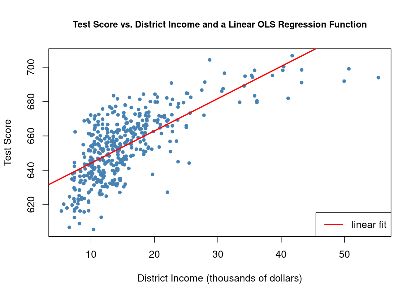
The plot shows that the linear regression line seems to overestimate the true relationship when income is either very high or very low and it tends to underestimates it for the middle income group. Luckily, Ordinary Least Squares (OLS) isn’t limited to linear regressions of the predictors. We have the flexibility to model test scores as a function of income and the square of income. This leads us to the following regression model:
TestScore_i = \beta_0 + \beta_1 \, income_i + \beta_2 \, income_i^2 + u_i which is a quadratic regression model. Here we treat income^2 as an additional explanatory variable.
In R, we can fit the model again with lm() but we have to use the ^ operator in conjunction with the function I() to add the quadratic term as an additional regressor to the argument formula. The reason is that the regression formula we pass to formula is converted to an object of the class formula, and for objects of this class, the operators +, -, * and ^ have a nonarithmetic interpretation. I() ensures that they are used as arithmetical operators (see ?I)
# fit the quadratic Model
quadratic_model <- lm(score ~ income + I(income^2), data = CASchools)

# obtain the model summary
coeftest(quadratic_model, vcov. = vcovHC, type = "HC1")
t test of coefficients:

               Estimate  Std. Error  t value  Pr(>|t|)
(Intercept) 607.3017435   2.9017544 209.2878 < 2.2e-16 ***
income        3.8509939   0.2680942  14.3643 < 2.2e-16 ***
I(income^2)  -0.0423084   0.0047803  -8.8505 < 2.2e-16 ***
---
Signif. codes:  0 '***' 0.001 '**' 0.01 '*' 0.05 '.' 0.1 ' ' 1
The estimated function is
\widehat{TestScore} = \underset{(2.90)}{607.3} \,+ \underset{(0.27)}{3.85} \, income_i - \underset{(0.0048)}{0.0423} \, income_i^2
We can test the hypothesis that the relationship between test scores and income is linear against the alternative that it is quadratic, by testing
H_0: \beta_2 = 0 \ \ vs. \ \ H_1: \beta_2 \neq 0 since \beta_2 = 0 would result in a simple linear equation and \beta_2 \neq 0 implies a quadratic relationship.
We can manually compute the t-value reported in the table as t =(\hat{\beta}_2 - 0)/SE(\hat{\beta}_2) = -0.042308/0.00478 = -8.85. With this t-value we can reject the null hypothesis at any common level of significance and we may conclude that the relationship is not linear. We could also have drawn the same conclusion by looking at the asterisks in the summary table, where we observe that the coefficient for the quadratic term is highly significant at the 0.1\% level (***).
We will now draw the same scatter plot as for the linear model and add the regression line for the quadratic model. Since abline() only plots straight lines, it cannot be used here, but we can use lines() function instead, which is suitable for plotting nonstraight lines (see ?lines). The most basic call of lines() is lines(x_values, y_values) where x_values and y_values are vectors of the same length that provide coordinates of the points to be sequentially connected by a line. This requires sorted coordinate pairs according to the X-values. We may use the function order() to sort the fitted values of score according to the observations of income, obtained from our quadratic model.
# draw a scatterplot of the observations for income and test score
plot(CASchools$income, CASchools$score,
     col  = "steelblue",
     pch = 20,
     xlab = "District Income (thousands of dollars)",
     ylab = "Test Score",
     main = "Estimated Linear and Quadratic Regression Functions")

# add a linear function to the plot
abline(linear_model, col = "green", lwd = 2)

# add quatratic function to the plot
order_id <- order(CASchools$income)

lines(x = CASchools$income[order_id],
      y = fitted(quadratic_model)[order_id],
      col = "red",
      lwd = 2)
legend("bottomright",legend=c("Linear Line","Quadratic Line"),
       lwd=2,col=c("green","red"))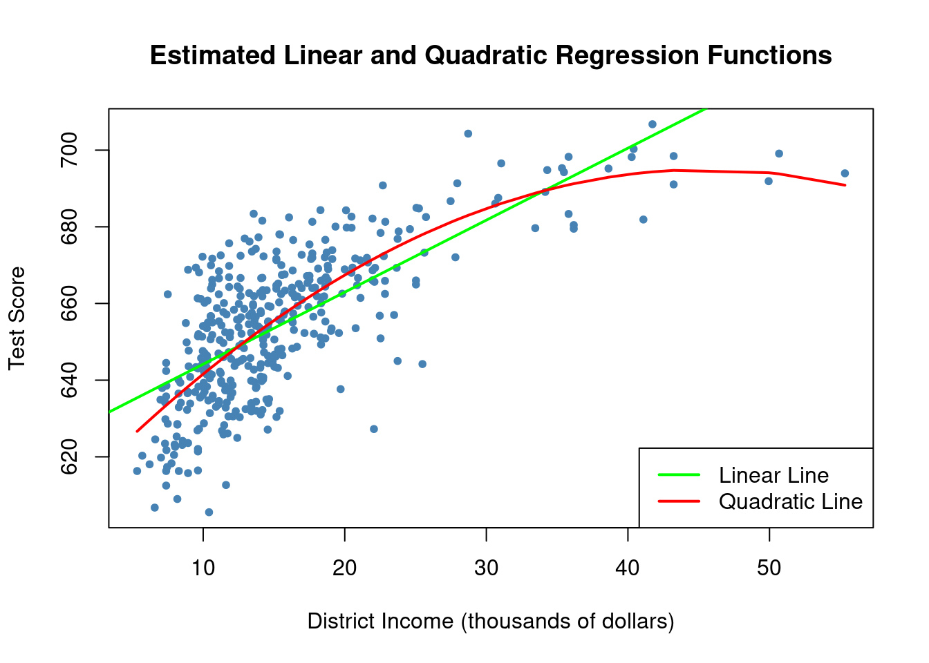
As the plot shows, the quadratic function appears to provide a better fit to the data compared to the linear function.
3.1 Polynomials
The method employed to derive a quadratic model can be extended to polynomial models of any degree r
Y_i = \beta_0 + \beta_1 X_i + \beta_2 X_i^2 + \ldots + \beta_r X_i^r + u_i
We can estimate polynomial models in R using the function poly(). The polynomial degrees (r) must be indicated into the degree argument of the function. For a cubic model:
The function poly() generates orthogonal polynomials that default to being orthogonal to the constant term. By setting raw = TRUE, we evaluate raw polynomials instead. For more information, refer to ?poly.
3.1.1 Joint Hypothesis Testing
A common dilemma in practice is selecting the optimal polynomial order. Similar to the quadratic regression model, we can test the null hypothesis suggesting that the true relationship is linear, in contrast to the alternative hypothesis proposing a polynomial relationship.
H_0: \beta_2 = 0, \beta_3 = 0, \ldots, \beta_r = 0 \quad \text{vs.} \quad H_1: \text{at least one } \, \beta_j \neq 0, \quad j = 2, \ldots, r.
This represents a joint null hypothesis with r-1 restrictions, which can be tested using the F-test previously described. The function linearHypothesis() facilitates such testing. For instance, we can test the null of a linear model against the alternative of a polynomial with a maximum degree r=3 as demonstrated below.
# test the hypothesis of a linear model against quadratic or cubic alternatives

# set up hypothesis matrix
R <- rbind(c(0, 0, 1, 0),
            c(0, 0, 0, 1))

# do the test
linearHypothesis(cubic_model,
                 hypothesis.matrix = R,
                 white.adj = "hc1")
Linear hypothesis test
Hypothesis:
poly(income, degree = 3, raw = TRUE)2 = 0
poly(income, degree = 3, raw = TRUE)3 = 0
Model 1: restricted model
Model 2: score ~ poly(income, degree = 3, raw = TRUE)
Note: Coefficient covariance matrix supplied.
Res.Df Df F Pr(>F)
1 418
2 416 2 37.691 9.043e-16 ***
---
Signif. codes: 0 '***' 0.001 '**' 0.01 '*' 0.05 '.' 0.1 ' ' 1We have created and supplied the hypothesis matrix R as the input argument hypothesis.matrix. This is convenient when the constraints involve several coefficients and when coefficients have long names, such as when using poly() (see summary(cubic_model)). The interpretation of the hypothesis matrix R by linearHypothesis() is best understood through matrix algebra. For our case with two linear constraints it would be as follows:
\begin{align*} R\beta &= s \\ \begin{pmatrix} 0 & 0 & 1 & 0 \\ 0 & 0 & 0 & 1 \end{pmatrix} \begin{pmatrix} \beta_0 \\ \beta_1 \\ \beta_2 \\ \beta_3 \end{pmatrix} &= \begin{pmatrix} 0 \\ 0 \end{pmatrix} \Rightarrow \begin{pmatrix} \beta_2 \\ \beta_3 \end{pmatrix} = \begin{pmatrix} 0 \\ 0 \end{pmatrix} \end{align*}
linearHypothesis() uses the zero vector for s by default, see ?linearHypothesis.
From the results of the joint hypothesis test, with a very small p-value, we can reject the null hypothesis of a linear relationship. However, we still face the challenge of choosing the right polynomial degree r. In other words, how many powers of X should be included in a polynomial regression. Increasing the degree r introduces more flexibility into the regression function, but adding more regressors can reduce the precision of the estimated coefficients.
While there is no general rule to select r, this could be determined by sequential testing, where individual hypotheses are tested sequentially in the following steps:
Estimate the polynomial regression model for a maximum value of r.
Use a t-test to test \beta_r = 0. If the null hypothesis is rejected, then X^r belongs in the regression equation.
If the null is accepted, X^r can be excluded from the model. Then repeat step 1 with order r-1 and test whether \beta_{r-1}=0. If the null is rejected, use a polynomial model of order r-1.
If the null is not rejected in step 3, continue this procedure until the coefficient on the highest power in your polynomial is statistically significant.
To choose the initial maximum value of r, Stock and Watson (2015) suggest to choose 2, 3 or 4 for applications on economic data, due to its usual smoothness (absence of jumps or “spikes).
We will apply this sequential testing to our cubic model reporting robust standard errors:
# test the hypothesis using robust standard errors
coeftest(cubic_model, vcov. = vcovHC, type = "HC1")
t test of coefficients:

                                         Estimate  Std. Error  t value
(Intercept)                            6.0008e+02  5.1021e+00 117.6150
poly(income, degree = 3, raw = TRUE)1  5.0187e+00  7.0735e-01   7.0950
poly(income, degree = 3, raw = TRUE)2 -9.5805e-02  2.8954e-02  -3.3089
poly(income, degree = 3, raw = TRUE)3  6.8549e-04  3.4706e-04   1.9751
                                       Pr(>|t|)
(Intercept)                           < 2.2e-16 ***
poly(income, degree = 3, raw = TRUE)1 5.606e-12 ***
poly(income, degree = 3, raw = TRUE)2  0.001018 **
poly(income, degree = 3, raw = TRUE)3  0.048918 *
---
Signif. codes:  0 '***' 0.001 '**' 0.01 '*' 0.05 '.' 0.1 ' ' 1
The estimated cubic regression function relating district income to test scores is
\widehat{TestScore} = \underset{(5.1)}{600.1} + \underset{(0.71)}{5.02} \, Income - \underset{(0.029)}{0.096} \, Income^2 + \underset{(0.00035)}{0.00069} \, Income^3
The t-statistic on Income^3 is 1.98, so the null hypothesis that the regression function is a quadratic is rejected against the alternative that it is a cubic at the 5\% level.
We can additionally test if the coefficients for Income^2 and Income^3 are jointly significant using a robust version of the F-test:
# perform robust F-test
linearHypothesis(cubic_model,
                 hypothesis.matrix = R,
                 vcov. = vcovHC, type = "HC1")
Linear hypothesis test
Hypothesis:
poly(income, degree = 3, raw = TRUE)2 = 0
poly(income, degree = 3, raw = TRUE)3 = 0
Model 1: restricted model
Model 2: score ~ poly(income, degree = 3, raw = TRUE)
Note: Coefficient covariance matrix supplied.
Res.Df Df F Pr(>F)
1 418
2 416 2 29.678 8.945e-13 ***
---
Signif. codes: 0 '***' 0.001 '**' 0.01 '*' 0.05 '.' 0.1 ' ' 1With a p-value below 0.001, we reject the null hypothesis that the regression function is linear against the alternative of a quadratic or cubic relationship.
3.1.2 Interpretation of coefficients
The coefficients in polynomial regressions do not have a simple interpretation. The best way to interpret them is to calculate the estimated effect on Y associated with a change in X for one or more values of X.
For example, if we would like to know the predicted change in test scores when income changes from 10 to 11 (thousand dollars) based on our estimated quadratic regression function
\widehat{TestScore} = 607.3 + 3.85 \, \text{Income} - 0.0423 \, \text{Income}^2
we would compute the \Delta \hat Y associated with that specific unit change in income using the following formula:
\widehat{\Delta Y} = (\hat{\beta}_0 + \hat{\beta}_1 \times 11 + \hat{\beta}_2 \times 11^2) - (\hat{\beta}_0 + \hat{\beta}_1 \times 10 + \hat{\beta}_2 \times 10^2)
We can compute \Delta \hat Y in R using predict()
# compute and assign the quadratic model
quadratic_model <- lm(score ~ income + I(income^2), data = CASchools)

# set up data for prediction
new_data <- data.frame(income = c(10, 11))

# do the prediction
Y_hat <- predict(quadratic_model, newdata = new_data)

# compute the difference
diff(Y_hat)
2
2.962517 The expected change in TestScore when increasing income from 10 to 11 (thousand dollars) is about 2.96 points. Note that, since the relationship is not linear, this unit change effect will vary depending on the pair of values of X selected. One way to notice this is by plotting the estimated quadratic regression function.
3.2 Logarithms
Another approach to express a nonlinear regression function involves using the natural logarithm of Y and/or X. Logarithms help convert variable changes into percentages, which is useful as many relationships are naturally described in terms of percentages. There are three different situations where logarithms are used: when X is transformed by taking its logarithm but Y is not; when Y is transformed to its logarithm but X is not; and when both Y and X are transformed to their logarithm.
3.2.1 Case I: X is in logarithms, Y is not.
In this case, sometimes referred to as a linear-log model, the regression model is
Y_i = \beta_0 + \beta_1 \ln(X_i) + u_i, \quad i = 1, \ldots, n.
As for polynomial regressions, there is no need to create the logged variable in advance, but we simply adjust the formula argument in lm() to log-transform the variable of interest.
# estimate a level-log model
LinearLog_model <- lm(score ~ log(income), data = CASchools)

# compute robust summary
coeftest(LinearLog_model,
         vcov = vcovHC, type = "HC1")
t test of coefficients:

            Estimate Std. Error t value  Pr(>|t|)
(Intercept) 557.8323     3.8399 145.271 < 2.2e-16 ***
log(income)  36.4197     1.3969  26.071 < 2.2e-16 ***
---
Signif. codes:  0 '***' 0.001 '**' 0.01 '*' 0.05 '.' 0.1 ' ' 1
The estimated regression model is
\widehat{TestScore} = \underset{(3.84)}{557.8} + \underset{(1.40)}{36.42} \, \ln (Income)
We plot this function
# draw a scatterplot
plot(score ~ income,
     col = "steelblue",
     pch = 20,
     data = CASchools,
     ylab="Score",
     xlab="Income",
     main = "Linear-Log Regression Line")

# add the linear-log regression line
order_id  <- order(CASchools$income)

lines(CASchools$income[order_id],
      fitted(LinearLog_model)[order_id],
      col = "red",
      lwd = 2)
legend("bottomright",legend = "Linear-log line",lwd = 2,col ="red")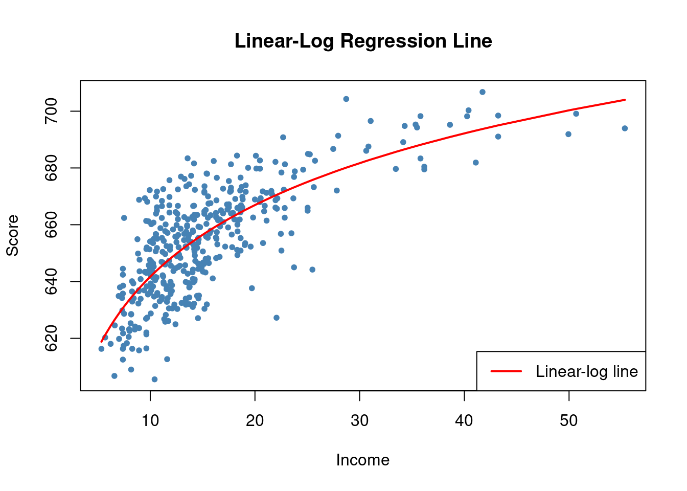
We can interpret \hat \beta_1 as follows: a 1\% increase in income is associated with an average increase in test scores of 0.01 \times 36.42 = 0.36 points. If we wanted to compute the change in TestScore of a one unit change in income, we would compute the \Delta \hat Y just as we did with polynomials.
3.2.2 Case II: Y is in logarithms, X is not
In this second case, the log-linear model, the regression function is
\ln (Y_i) = \beta_0 + \beta_1 X_i + u_i, \quad i = 1, \ldots, n.
# estimate a log-linear model
LogLinear_model <- lm(log(score) ~ income, data = CASchools)

# obtain a robust coefficient summary
coeftest(LogLinear_model,
         vcov = vcovHC, type = "HC1")
t test of coefficients:

              Estimate Std. Error  t value  Pr(>|t|)
(Intercept) 6.43936234 0.00289382 2225.210 < 2.2e-16 ***
income      0.00284407 0.00017509   16.244 < 2.2e-16 ***
---
Signif. codes:  0 '***' 0.001 '**' 0.01 '*' 0.05 '.' 0.1 ' ' 1
The estimated regression function is
\ln (\widehat{TestScore}) = \underset{(0.003)}{6.439} + \underset{(0.0002)}{0.00284} \, Income
An increase in income of one unit (\$1000) is associated with an average increase in TestScore of 100 \times 0.00284 = 0.284\%
Note that when the dependent variable is in logarithms, one cannot use e^{\log(\cdot)} to transform predictions back to the original scale, as pointed by Stock and Watson (2015).
3.2.3 Case III: X and Y are in logarithms
The log-log regression model is
\ln (Y_i) = \beta_0 + \beta_1 \ln (X_i) + u_i, \quad i = 1, \ldots, n.
# estimate the log-log model
LogLog_model <- lm(log(score) ~ log(income), data = CASchools)

# print robust coefficient summary
coeftest(LogLog_model,
         vcov = vcovHC, type = "HC1")
t test of coefficients:

             Estimate Std. Error  t value  Pr(>|t|)
(Intercept) 6.3363494  0.0059246 1069.501 < 2.2e-16 ***
log(income) 0.0554190  0.0021446   25.841 < 2.2e-16 ***
---
Signif. codes:  0 '***' 0.001 '**' 0.01 '*' 0.05 '.' 0.1 ' ' 1
The estimated log-log regression function is
\ln (\widehat{TestScore}) = \underset{(0.006)}{6.336} + \underset{(0.002)}{0.0554} \, \ln(Income)
A 1\% increase in Income is associated with an average increase in TestScore of 0.055\%
We now plot the log-linear and the log-log regression models together
# generate a scatterplot
plot(log(score) ~ income,
     col = "steelblue",
     pch = 20,
     data = CASchools,
     ylab="log(Score)",
     xlab="Income",
     main = "Log-Linear Regression Function")

# add the log-linear regression line
order_id  <- order(CASchools$income)

lines(CASchools$income[order_id],
      fitted(LogLinear_model)[order_id],
      col = "red",
      lwd = 2)

# add the log-log regression line
lines(sort(CASchools$income),
      fitted(LogLog_model)[order(CASchools$income)],
      col = "green",
      lwd = 2)

# add a legend
legend("bottomright",
       legend = c("log-linear model", "log-log model"),
       lwd = 2,
       col = c("red", "green"))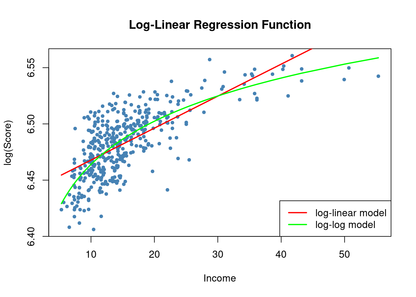
3.2.4 Comparing logarithmic specifications
Which of the log regression models best fits the data? The \bar {R^2} can be used to compare the log-linear and log-log models. Similarly, the \bar {R^2} can be used to compare the linear-log regression and the linear regression of Y against X. But unfortunately, the \bar {R^2} cannot be used to compare the linear-log and the log-log model because their dependent variables are different (one is Y, the other one is \ln(Y)). Because of this problem, the best thing to do in a particular application is to decide, using economic theory and experts’ knowledge of the problem, whether it makes sense to specify Y in logarithms.
# compute the adj. R^2 for the nonlinear models
adj_R2 <-rbind("quadratic" = summary(quadratic_model)$adj.r.squared,
               "cubic" = summary(cubic_model)$adj.r.squared,
               "LinearLog" = summary(LinearLog_model)$adj.r.squared,
               "LogLinear" = summary(LogLinear_model)$adj.r.squared,
               "LogLog" = summary(LogLog_model)$adj.r.squared)

# assign column names
colnames(adj_R2) <- "adj_R2"

adj_R2
adj_R2
quadratic 0.5540444
cubic 0.5552279
LinearLog 0.5614605
LogLinear 0.4970106
LogLog 0.5567251From those models where the dependent variable is TestScore, we observe a very similar adjusted fit. We can compare the cubic and the linear-log model by plotting their estimated regression functions.
# generate a scatterplot
plot(score ~ income,
     data = CASchools,
     col = "steelblue",
     pch = 20,
     ylab="Score",
     xlab="Income",
     main = "Linear-Log and Cubic Regression Functions")

# add the linear-log regression line
order_id  <- order(CASchools$income)

lines(CASchools$income[order_id],
      fitted(LinearLog_model)[order_id],
      col = "darkgreen",
      lwd = 2)

# add the cubic regression line
lines(x = CASchools$income[order_id],
      y = fitted(cubic_model)[order_id],
      col = "red",
      lwd = 2)
# add a legend
legend("bottomright",
       legend = c("Linear-Log model", "Cubic model"),
       lwd = 2,
       col = c("darkgreen", "red"))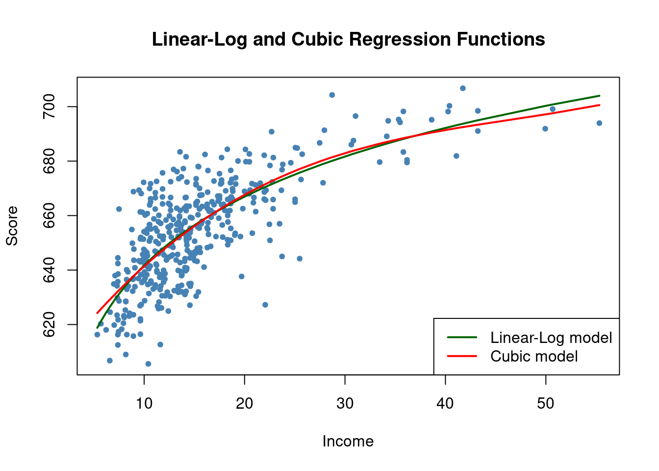
We appreciate a nearly identical look for both models, although we may prefer the linear-log model for simplicity, since it does not include higher-degree polynomials.
3.3 Interactions Between Independent Variables
Sometimes it is interesting to learn how the effect on Y of a change in an independent variable depends on the value of another independent variable. For example, we may ask if districts with many English learners benefit differently from a decrease in the student-teacher ratio compared to those with fewer English learning students. We can assess this by using a multiple regression model and including an interaction term.
We consider three cases: when both independent variables are binary, when one is binary and the other is continuous, and when both are continuous.
3.3.1 Interactions Between Two Binary Variables
Let
\begin{equation*} \begin{aligned} \text{HiSTR} &= \begin{cases} 1, & \text{if } \text{STR} \geq 20 \\ 0, & \text{else} \end{cases} \\ \text{HiEL} &= \begin{cases} 1, & \text{if } \text{english} \geq 10 \\ 0, & \text{else} \end{cases} \end{aligned} \end{equation*}
In R, we construct this dummies as follows
# append HiSTR to CASchools
CASchools$HiSTR <- as.numeric(CASchools$STR >= 20)

# append HiEL to CASchools
CASchools$HiEL <- as.numeric(CASchools$english >= 10)
We now estimate the model
TestScore = \beta_0 + \beta_1 \, HiSTR + \beta_2 \, HiEL + \beta_3 \, HiSTR \times HiEL + u_i.
We can simply indicate HiEL * HiSTR inside the lm() formula to add the interaction term to the model. Note that this adds HiEL, HiSTR and their interaction as regressors, whereas indicating HiEL:HiSTR only adds the interaction term.
# estimate the model with a binary interaction term
bi_model <- lm(score ~ HiSTR * HiEL, data = CASchools)

# print a robust summary of the coefficients
coeftest(bi_model, vcov. = vcovHC, type = "HC1")
t test of coefficients:

            Estimate Std. Error  t value  Pr(>|t|)
(Intercept) 664.1433     1.3881 478.4589 < 2.2e-16 ***
HiSTR        -1.9078     1.9322  -0.9874    0.3240
HiEL        -18.3155     2.3340  -7.8472 3.634e-14 ***
HiSTR:HiEL   -3.2601     3.1189  -1.0453    0.2965
---
Signif. codes:  0 '***' 0.001 '**' 0.01 '*' 0.05 '.' 0.1 ' ' 1
The estimated regression model is
\widehat{TestScore} = \underset{(1.39)}{664.1} - \underset{(1.93)}{1.9} \, \text{HiSTR} - \underset{(2.33)}{18.3} \, \text{HiEL} - \underset{(3.12)}{3.3} \, (\text{HiSTR} \times \text{HiEL})
According to this model, when moving from a school district with a low student-teacher ratio to one with a high ratio, the average effect on test scores depends on the percentage of English learners (HiEL), and can be computed as -1.9 - 3.3 \times HiEL. This is, for districts with fewer English learners (HiEL = 0), the expected decrease in test scores is 1.9 points. However, for districts with a higher proportion of English learners (HiEL = 1), the predicted decrease in test scores is 1.9 + 3.3 = 5.2 points.
We can estimate the mean test score for each possible combination of the included binary variables
# estimate means for all combinations of HiSTR and HiEL

# 1.
predict(bi_model, newdata = data.frame("HiSTR" = 0, "HiEL" = 0))
1
664.1433 # 2.
predict(bi_model, newdata = data.frame("HiSTR" = 0, "HiEL" = 1)) 1
645.8278 # 3.
predict(bi_model, newdata = data.frame("HiSTR" = 1, "HiEL" = 0)) 1
662.2354 # 4.
predict(bi_model, newdata = data.frame("HiSTR" = 1, "HiEL" = 1)) 1
640.6598 We verify that these predictions are differences in the coefficient estimates presented in the regression equation
\begin{align*} \widehat{TestScore} = \hat{\beta}_0 = 664.1 &\Leftrightarrow HiSTR = 0, \quad HiEL = 0. \\ \widehat{TestScore} = \hat{\beta}_0 + \hat{\beta}_2 = 664.1 - 18.3 = 645.8 &\Leftrightarrow HiSTR = 0, \quad HiEL = 1. \\ \widehat{TestScore} = \hat{\beta}_0 + \hat{\beta}_1 = 664.1 - 1.9 = 662.2 &\Leftrightarrow HiSTR = 1, \quad HiEL = 0. \\ \widehat{TestScore} = \hat{\beta}_0 + \hat{\beta}_1 + \hat{\beta}_2 + \hat{\beta}_3 = 664.1 - 1.9 - 18.3 - 3.3 = 640.6 &\Leftrightarrow HiSTR = 1, \quad HiEL = 1. \end{align*}
3.3.2 Interactions Between a Continuous and a Binary Variable
This specification where the interaction term includes a continuous variable (X_i) and a binary variable (D_i) allows for the slope to depend on the binary variable. There are three different possibilities:
- Different intercepts, same slope:
Y_i = \beta_0 + \beta_1 X_i + \beta_2 D_i + u_i
- Different intercepts and slopes:
Y_i = \beta_0 + \beta_1 X_i + \beta_2 D_i + \beta_3 \times (X_i \times D_i) + u_i
- Same intercept, different slopes:
Y_i = \beta_0 + \beta_1 X_i + \beta_2 (X_i \times D_i) + u_i. Does the effect on test scores of cutting the student-teacher ratio depend on whether the percentage of students still learning English is high or low? One way to answer this question is to use a specification that allows for two different regression lines, depending on whether there is a high or a low percentage of English learners. This is achieved using the different intercept/different slope specification. We estimate the regression model
\widehat{TestScore}_i = \beta_0 + \beta_1 \, STR_i + \beta_2 \, HiEL_i + \beta_2 \, (STR_i \times HiEL_i) + u_i
# estimate the model
bci_model <- lm(score ~ STR + HiEL + STR * HiEL, data = CASchools)

# print robust summary of coefficients
coeftest(bci_model, vcov. = vcovHC, type = "HC1")
t test of coefficients:

             Estimate Std. Error t value Pr(>|t|)
(Intercept) 682.24584   11.86781 57.4871   <2e-16 ***
STR          -0.96846    0.58910 -1.6440   0.1009
HiEL          5.63914   19.51456  0.2890   0.7727
STR:HiEL     -1.27661    0.96692 -1.3203   0.1875
---
Signif. codes:  0 '***' 0.001 '**' 0.01 '*' 0.05 '.' 0.1 ' ' 1
\widehat{TestScore} = \underset{(11.87)}{682.2} - \underset{(0.59)}{0.97} \, STR + \underset{(19.51)}{5.6} \, HiEL - \underset{(0.97)}{1.28} \, (STR \times HiEL).
The estimated regression line for districts with a low fraction of English learners (HiEL=0) is
\widehat{TestScore} = 682.2 - 0.97 \, STR_i while the one for districts with a high fraction of English learners (HiEL=1) is
\begin{align*} \widehat{TestScore} &= 682.2 + 5.6 - 0.97 \, STR_i - 1.28 \, STR_i \\ &= 687.8 - 2.25 \, STR_i. \end{align*}
The expected rise in test scores after decreasing the student-teacher ratio by one unit is roughly 0.97 points in districts with a low proportion of English learners, but 2.25 points in districts with a high concentration of English learners. The coefficient on the interaction term, “STR \times HiEL”, indicates that the contrast between these effects amounts to 1.28 points.
We now plot both regression lines from the model by using different colors to differentiate each of the STR levels.
# identify observations with english >= 10
id <- CASchools$english >= 10

# plot observations with HiEL = 0 as red dots
plot(CASchools$STR[!id], CASchools$score[!id],
     xlim = c(0, 27),
     ylim = c(600, 720),
     pch = 20,
     col = "red",
     main = "",
     xlab = "Class Size",
     ylab = "Test Score")

# plot observations with HiEL = 1 as green dots
points(CASchools$STR[id], CASchools$score[id],
     pch = 20,
     col = "green")

# read out estimated coefficients of bci_model
coefs <- bci_model$coefficients

# draw the estimated regression line for HiEL = 0
abline(coef = c(coefs[1], coefs[2]),
       col = "red",
       lwd = 1.5)

# draw the estimated regression line for HiEL = 1
abline(coef = c(coefs[1] + coefs[3], coefs[2] + coefs[4]),
       col = "green",
       lwd = 1.5 )

# add a legend to the plot
legend("topleft",
       pch = c(20, 20),
       col = c("red", "green"),
       legend = c("HiEL = 0", "HiEL = 1"))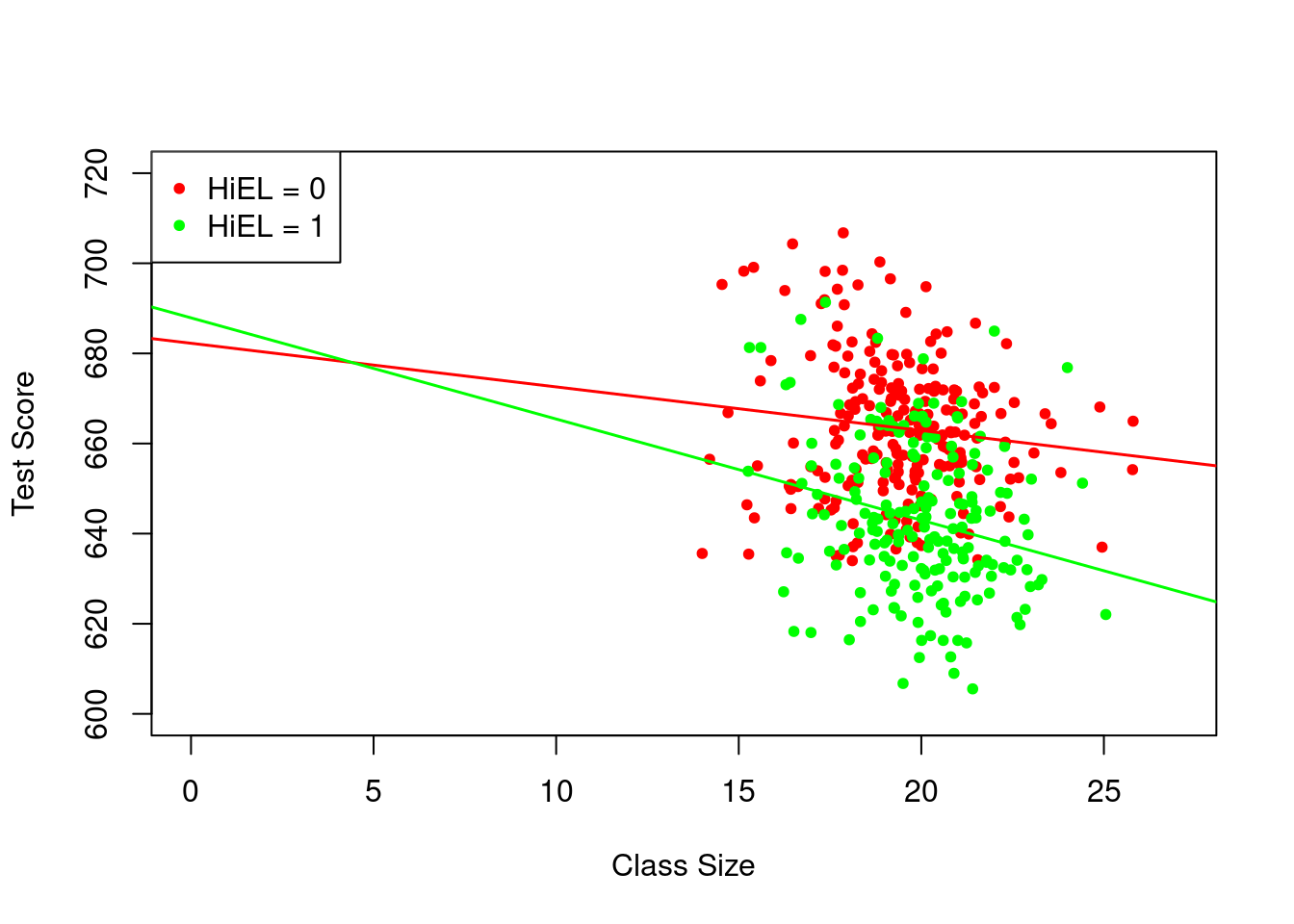
3.3.3 Interactions Between Two Continuous Variables
Let’s now examine the interaction between the continuous variables student-teacher ratio (STR) and the percentage of English learners (english).
# estimate regression model including the interaction between 'english' and 'STR'
cci_model <- lm(score ~ STR + english + english * STR, data = CASchools)

# print summary
coeftest(cci_model, vcov. = vcovHC, type = "HC1")
t test of coefficients:

               Estimate  Std. Error t value Pr(>|t|)
(Intercept) 686.3385268  11.7593466 58.3654  < 2e-16 ***
STR          -1.1170184   0.5875136 -1.9013  0.05796 .
english      -0.6729119   0.3741231 -1.7986  0.07280 .
STR:english   0.0011618   0.0185357  0.0627  0.95005
---
Signif. codes:  0 '***' 0.001 '**' 0.01 '*' 0.05 '.' 0.1 ' ' 1
The estimated regression function is
\widehat{TestScore} = \underset{(11.76)}{686.3} - \underset{(0.59)}{1.12} \, STR - \underset{(0.37)}{0.67} \, english + \underset{(0.02)}{0.0012} \, (STR \times english).
Before proceeding with the interpretations, let us explore the quartiles of english
summary(CASchools$english) Min. 1st Qu. Median Mean 3rd Qu. Max.
0.000 1.941 8.778 15.768 22.970 85.540 When the percentage of English learners is at the median (english = 8.778), the slope of the line is estimated to be (-1.12 + 0.0012 * 8.778 = -1.12). When the percentage of English learners is at the 75th percentile (english = 22.97), this line is estimated to be slightly flatter, with a slope of -1.12 + 0.0012 * 22.97 = -1.09. In other words, for a district with 8.78\% English learners, the estimated effect of a one-unit reduction in the student-teacher ratio is to increase on average test scores by 1.11 points, but for a district with 23\% English learners, reducing the student-teacher ratio by one unit is predicted to increase test scores on average by 1.09 points. However, it is important to note from the output of coeftest() that the estimated coefficient on the interaction term (\beta_3) is not statistically significant at the 10\% level, so we cannot reject the null hypothesis H_0 : \beta_3 = 0.
3.4 Nonlinear Effects on Test Scores of the Student-Teacher Ratio
This section examines three key questions about test scores and the student-teacher ratio. First, it explores if reducing the student-teacher ratio affects test scores differently based on the number of English learners, even when considering economic differences across districts. Second, it investigates if this effect varies depending on the student-teacher ratio. Lastly, it aims to determine the expected impact on test scores when the student-teacher ratio decreases by two students per teacher, considering both economic factors and potential nonlinear relationships.
We will answer these questions considering the previously explained nonlinear regression specifications, extended to include two measures of the economic background of the students: the percentage of students eligible for a subsidized lunch (lunch) and the logarithm of average district income (ln(income)). The logarithm of district income is used following our previous empirical analysis, which suggested that this specification captures the nonlinear relationship between scores and income. We leave out the expenditure per pupil (expenditure) from our analysis because including it would suggest that spending changes with the student-teacher ratio (in other words, we would not be holding expenditures per pupil constant).
We will consider 7 different model specifications:
\begin{align*} TestScore_i &= \beta_0 + \beta_1 \, STR_i + \beta_2 \, english_i + \beta_3 \, lunch_i + u_i. \\[6pt] TestScore_i &= \beta_0 + \beta_1 \, STR_i + \beta_2 \, english_i + \beta_3 \ln(income_i) + u_i. \\[6pt] TestScore_i &= \beta_0 + \beta_1 \, STR_i + \beta_2 \, HiEL_i + \beta_3 \, (HiEL_i \times STR_i) + u_i. \\[6pt] TestScore_i &= \beta_0 + \beta_1 \, STR_i + \beta_2 \, HiEL_i + \beta_3 \, (HiEL_i \times STR_i) + \beta_4 \, lunch_i + \beta_5 \ln(income_i) + u_i. \\[6pt] TestScore_i &= \beta_0 + \beta_1 \, STR_i + \beta_2 \, STR^2_i + \beta_3 \, HiEL_i + \beta_4 \, lunch_i + \beta_5 \ln(income_i) + u_i. \\[6pt] TestScore_i &= \beta_0 + \beta_1 \, STR_i + \beta_2 \, STR^2_i + \beta_3 \, STR^3_i + \beta_4 \, HiEL_i + \beta_5 \, (HiEL_i \times STR_i) \\ &+ \beta_6 \, (HiEL_i \times STR^2_i) + \beta_7 \, (HiEL_i \times STR^3_i) + \beta_8 \, lunch_i + \beta_9 \ln(income_i) + u_i. \\[6pt] TestScore_i &= \beta_0 + \beta_1 \, STR_i + \beta_2 \, STR^2_i + \beta_3 \, STR^3_i + \beta_4 \, english_i + \beta_5 \, lunch_i + \beta_6 \ln(income_i) + u_i. \end{align*}
# estimate all models
TS_mod1 <- lm(score ~ STR + english + lunch, data = CASchools)

TS_mod2 <- lm(score ~ STR + english + lunch + log(income), data = CASchools)

TS_mod3 <- lm(score ~ STR + HiEL + HiEL:STR, data = CASchools)

TS_mod4 <- lm(score ~ STR + HiEL + HiEL:STR + lunch + log(income), data = CASchools)

TS_mod5 <- lm(score ~ STR + I(STR^2) + I(STR^3) + HiEL + lunch + log(income),
    data = CASchools)

TS_mod6 <- lm(score ~ STR + I(STR^2) + I(STR^3) + HiEL + HiEL:STR + HiEL:I(STR^2) +
    HiEL:I(STR^3) + lunch + log(income), data = CASchools)

TS_mod7 <- lm(score ~ STR + I(STR^2) + I(STR^3) + english + lunch + log(income),
    data = CASchools)
We could use summary() to report the estimates of each model, but stargazer() conveniently reports the results of all models in a tabular form, which is more practical when comparing models.
# gather robust standard errors in a list
rob_se <- list(sqrt(diag(vcovHC(TS_mod1, type = "HC1"))),
               sqrt(diag(vcovHC(TS_mod2, type = "HC1"))),
               sqrt(diag(vcovHC(TS_mod3, type = "HC1"))),
               sqrt(diag(vcovHC(TS_mod4, type = "HC1"))),
               sqrt(diag(vcovHC(TS_mod5, type = "HC1"))),
               sqrt(diag(vcovHC(TS_mod6, type = "HC1"))),
               sqrt(diag(vcovHC(TS_mod7, type = "HC1"))))

# generate a LaTeX table of regression outputs
stargazer(TS_mod1, TS_mod2, TS_mod3, TS_mod4,
          TS_mod5, TS_mod6, TS_mod7,
          digits = 3,
          type = "text",
          header = FALSE,
          dep.var.caption = "Dependent Variable: Test Score",
          se = rob_se,
          model.numbers = FALSE,
          column.labels = c("(1)", "(2)", "(3)", "(4)", "(5)", "(6)", "(7)"))
=================================================================================================================================================================================================
                                                                                           Dependent Variable: Test Score
                    -----------------------------------------------------------------------------------------------------------------------------------------------------------------------------
                                                                                                        score
                              (1)                      (2)                      (3)                     (4)                      (5)                      (6)                      (7)
-------------------------------------------------------------------------------------------------------------------------------------------------------------------------------------------------
STR                        -0.998***                -0.734***                 -0.968                   -0.531                 64.339***                83.702***                65.285***
                            (0.270)                  (0.257)                  (0.589)                 (0.342)                  (24.861)                 (28.497)                 (25.259)

english                    -0.122***                -0.176***                                                                                                                   -0.166***
                            (0.033)                  (0.034)                                                                                                                     (0.034)

I(STR2)                                                                                                                       -3.424***                -4.381***                -3.466***
                                                                                                                               (1.250)                  (1.441)                  (1.271)

I(STR3)                                                                                                                        0.059***                 0.075***                 0.060***
                                                                                                                               (0.021)                  (0.024)                  (0.021)

lunch                      -0.547***                -0.398***                                        -0.411***                -0.420***                -0.418***                -0.402***
                            (0.024)                  (0.033)                                          (0.029)                  (0.029)                  (0.029)                  (0.033)

log(income)                                         11.569***                                        12.124***                11.748***                11.800***                11.509***
                                                     (1.819)                                          (1.798)                  (1.771)                  (1.778)                  (1.806)

HiEL                                                                           5.639                   5.498                  -5.474***                816.076**
                                                                             (19.515)                 (9.795)                  (1.034)                 (327.674)

STR:HiEL                                                                      -1.277                   -0.578                                          -123.282**
                                                                              (0.967)                 (0.496)                                           (50.213)

I(STR2):HiEL                                                                                                                                            6.121**
                                                                                                                                                        (2.542)

I(STR3):HiEL                                                                                                                                            -0.101**
                                                                                                                                                        (0.043)

Constant                   700.150***               658.552***              682.246***               653.666***                252.050                  122.353                  244.809
                            (5.568)                  (8.642)                 (11.868)                 (9.869)                 (163.634)                (185.519)                (165.722)

-------------------------------------------------------------------------------------------------------------------------------------------------------------------------------------------------
Observations                  420                      420                      420                     420                      420                      420                      420
R2                           0.775                    0.796                    0.310                   0.797                    0.801                    0.803                    0.801
Adjusted R2                  0.773                    0.794                    0.305                   0.795                    0.798                    0.799                    0.798
Residual Std. Error     9.080 (df = 416)         8.643 (df = 415)        15.880 (df = 416)        8.629 (df = 414)         8.559 (df = 413)         8.547 (df = 410)         8.568 (df = 413)
F Statistic         476.306*** (df = 3; 416) 405.359*** (df = 4; 415) 62.399*** (df = 3; 416) 325.803*** (df = 5; 414) 277.212*** (df = 6; 413) 185.777*** (df = 9; 410) 276.515*** (df = 6; 413)
=================================================================================================================================================================================================
Note:                                                                                                                                                                 *p<0.1; **p<0.05; ***p<0.01
What can be concluded from the results presented?
First, we we see the estimated coefficient on STR is highly significant in all models except from specifications (3) and (4). When we add log(income) to model (1) in the second specification, all coefficients remain highly significant while the coefficient on the new regressor is also statistically significant at the 1\% level. Additionally, the coefficient on STR is now 0.27 higher than in model (1), suggesting a possible mitigation of omitted variable bias when including ln(income) as regressor. For these reasons, it makes sense to keep this variable in other models too.
Models (3) and (4) include the interaction term between STR and HiEL, first without control variables in the third specification and then controlling for economic factors in the fourth. The estimated coefficient for the interaction term is not significant at any common level in any of these models, nor is the coefficient on the dummy variable HiEL. Hence, despite accounting for economic factors, we cannot reject the null hypotheses that the impact of the student-teacher ratio on test scores remains consistent across districts with high and low proportions of English learning students.
In regression (5) we have included quadratic and cubic terms for STR, while omitting the interaction term between STR and HiEL, since it was not significant in specification (4). The results indicate high levels of significance for these estimated coefficients and we can therefore assume the presence of a nonlinear effect of the student-teacher ration on test scores. This could be also verified with an F-test of H_0: \beta_2 = \beta_3 =0.
Regression (6) delves deeper into examining whether the proportion of English learners influences the student-teacher ratio, incorporating the interaction terms HiEL\times STR, HiEL\times STR^2 and HiEL\times STR^3. Each individual t-test confirms significant effects. To validate this, we perform a robust F-test to assess H_0: \beta_5 = \beta_6 = \beta_7 =0.
# check joint significance of the interaction terms
linearHypothesis(TS_mod6,
                 c("STR:HiEL=0", "I(STR^2):HiEL=0", "I(STR^3):HiEL=0"),
                 vcov. = vcovHC, type = "HC1")
Linear hypothesis test
Hypothesis:
STR:HiEL = 0
I(STR^2):HiEL = 0
I(STR^3):HiEL = 0
Model 1: restricted model
Model 2: score ~ STR + I(STR^2) + I(STR^3) + HiEL + HiEL:STR + HiEL:I(STR^2) +
HiEL:I(STR^3) + lunch + log(income)
Note: Coefficient covariance matrix supplied.
Res.Df Df F Pr(>F)
1 413
2 410 3 2.1885 0.08882 .
---
Signif. codes: 0 '***' 0.001 '**' 0.01 '*' 0.05 '.' 0.1 ' ' 1With a p-value of 0.08882 we can just reject the null hypothesis at the 10\% level. This provides tentative evidence that the regression functions are different for districts with high and low percentages of English learners, but this will be further explored later.
In model (7), we employ a continuous measure for the proportion of English learners instead of a dummy variable (thus omitting interaction terms). We note minimal alterations in the coefficient estimates for the remaining regressors. Consequently, we infer that the findings observed in model (5) are robust and not influenced significantly by the method used to measure the percentage of English learners.
For better interpretation, we now plot the nonlinear specifications (2), (5) and (7) along with a scatterplot of the data, setting all regressors except STR to their sample averages. The plotted regression functions represent the predicted value of test scores as a function of the student-teacher ratio, holding fixed other values of the independent variables in the regression.
# scatterplot
plot(CASchools$STR,
     CASchools$score,
     xlim = c(12, 28),
     ylim = c(600, 740),
     pch = 20,
     col = "gray",
     xlab = "Student-Teacher Ratio",
     ylab = "Test Score")

# add a legend
legend("top",
       legend = c("Linear Regression (2)",
                  "Cubic Regression (5)",
                  "Cubic Regression (7)"),
       cex = 0.6,
       ncol = 3,
       lty = c(1, 1, 2),
       col = c("blue", "red", "black"))

# data for use with predict()
new_data <- data.frame("STR" = seq(16, 24, 0.05),
                       "english" = mean(CASchools$english),
                       "lunch" = mean(CASchools$lunch),
                       "income" = mean(CASchools$income),
                       "HiEL" = mean(CASchools$HiEL))

# add estimated regression function for model (2)
fitted <- predict(TS_mod2, newdata = new_data)

lines(new_data$STR,
      fitted,
      lwd = 1.5,
      col = "blue")

# add estimated regression function for model (5)
fitted <- predict(TS_mod5, newdata = new_data)

lines(new_data$STR,
      fitted,
      lwd = 1.5,
      col = "red")

# add estimated regression function for model (7)
fitted <- predict(TS_mod7, newdata = new_data)

lines(new_data$STR,
      fitted,
      col = "black",
      lwd = 1.5,
      lty = 2)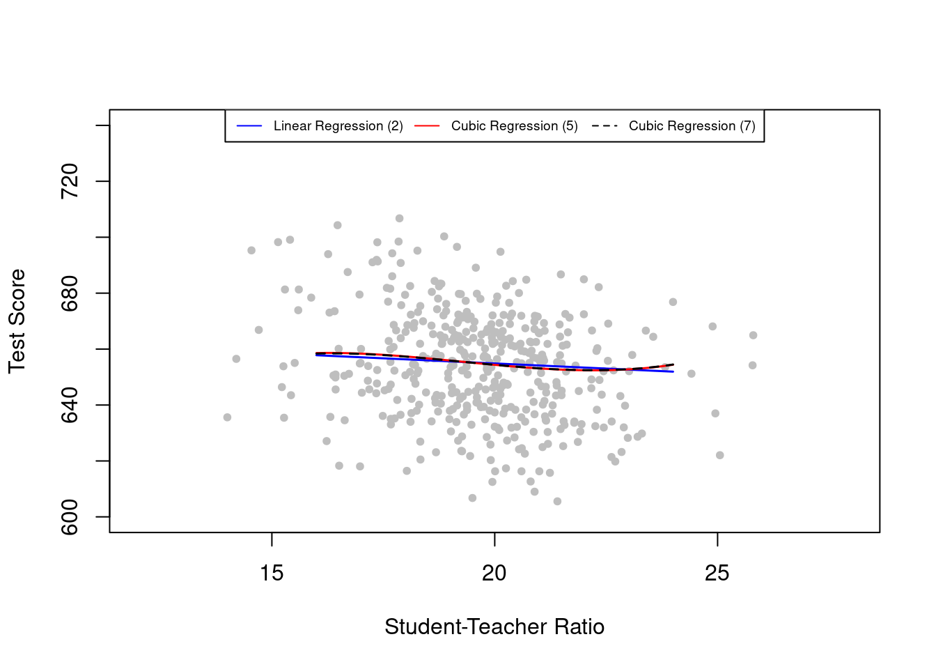
Cubic regressions (5) and (7) are represented by almost identical lines, and remarkably, all three estimated regression functions are close to one another. This may indicate that the relation between test scores and the student-teacher ratio has just a small amount of nonlinearity.
Regression (6) suggested that the cubic regression functions relating test scores and STR might depend on whether the percentage of English learners in the district is large or small, but the null was just rejected at the 10\% level. We can further explore this by plotting the two estimated regression functions from this model and assessing the differences. Districts with low percentages of English learners (HiEL = 0) will be shown by gray dots, and districts with HiEL =1 by colored dots. We use plot() and points() to color observations depending on HiEL, and we will make the predictions using the sample averages for all regressors except for STR, just as before.
# draw scatterplot

# observations with HiEL = 0
plot(CASchools$STR[CASchools$HiEL == 0],
     CASchools$score[CASchools$HiEL == 0],
     xlim = c(12, 28),
     ylim = c(600, 730),
     pch = 20,
     col = "gray",
     xlab = "Student-Teacher Ratio",
     ylab = "Test Score")

# observations with HiEL = 1
points(CASchools$STR[CASchools$HiEL == 1],
       CASchools$score[CASchools$HiEL == 1],
       col = "steelblue",
       pch = 20)

# add a legend
legend("top",
       legend = c("Regression (6) with HiEL=0", "Regression (6) with HiEL=1"),
       cex = 0.7,
       ncol = 2,
       lty = c(1, 1),
       col = c("green", "red"))

# data for use with 'predict()'
new_data <- data.frame("STR" = seq(12, 28, 0.05),
                       "english" = mean(CASchools$english),
                       "lunch" = mean(CASchools$lunch),
                       "income" = mean(CASchools$income),
                       "HiEL" = 0)

# add estimated regression function for model (6) with HiEL=0
fitted <- predict(TS_mod6, newdata = new_data)

lines(new_data$STR,
      fitted,
      lwd = 1.5,
      col = "green")

# add estimated regression function for model (6) with HiEL=1
new_data$HiEL <- 1

fitted <- predict(TS_mod6, newdata = new_data)

lines(new_data$STR,
      fitted,
      lwd = 1.5,
      col = "red")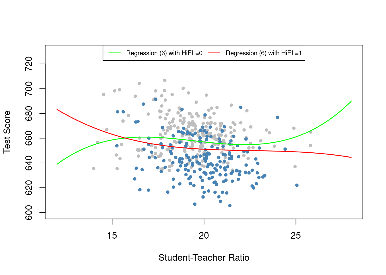
The plot shows that the difference between both isn’t of practical importance in reality. It’s a good example of why we need to be careful when understanding nonlinear models. Even though the two lines on the graph look different, they have almost the same slope between student-teacher ratios of 17 to 23. Since most of the data falls within this range, we can ignore any complicated relationships between the fraction of English learners and the student-teacher ratio. The two regression functions differ for student-teacher ratios below 17. However, we should be cautious not to draw conclusions beyond what is warranted. Districts with student-teacher ratios less than 16.5 make up only 6\% of the total observations. Therefore, any discrepancies between the nonlinear regression functions primarily come from differences in these few districts with extremely low student-teacher ratios.
Additionally, the model is less accurate at the very low and very high ends of the data, since there aren’t many observations there. This is a common problem with cubic functions - they can behave strangely at extreme values, as we can see in the graph of f(x)=x^3.
# Define the range of x values
x <- seq(-10, 10, by = 0.1)

# Calculate the corresponding y values using the cubic function
y <- x^3

# Plot the cubic function
plot(x, y, type = "l", col = "blue", lwd = 2,
     xlab = "x", ylab = "f(x)", main = "Plot of Cubic Function f(x) = x^3")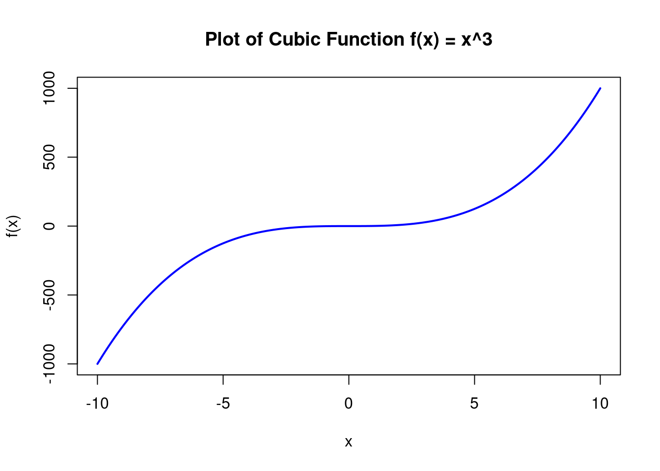
All in all, we conclude that the effect on test scores of a change in the student-teacher ratio does not depend on the percentage of English learners for the range of student-teacher ratios for which we have the most data.
3.4.1 Conclusions
We can now address the initial questions raised in this section:
First, in the linear models, the impact of the percentage of English learners on changes in test scores due to variations in the student-teacher ratio is minimal, a conclusion that holds true even after accounting for students’ economic backgrounds. Although the cubic specification (6) suggests that the relationship between student-teacher ratio and test scores is influenced by the proportion of English learners, the magnitude of this influence is not significant.
Second, while controlling for students’ economic backgrounds, we identify nonlinearities in the association between student-teacher ratio and test scores.
Lastly, under the linear specification (2), a reduction of two students per teacher in the student-teacher ratio is projected to increase test scores by approximately 1.46 points. As this model is linear, this effect remains consistent regardless of class size. For instance, assuming a student-teacher ratio of 20, the nonlinear model (5) indicates that the reduction in student-teacher ratio would lead to an increase in test scores by
64.33 \cdot 18 + 18^2 \cdot (-3.42) + 18^3 \cdot (0.059) - (64.33 \cdot 20 + 20^2 \cdot (-3.42) + 20^3 \cdot (0.059)) \approx 3.3 points. If the ratio was 22, a reduction to 20 leads to a predicted improvement in test scores of
64.33 \cdot 20 + 20^2 \cdot (-3.42) + 20^3 \cdot (0.059) - (64.33 \cdot 22 + 22^2 \cdot (-3.42) + 22^3 \cdot (0.059)) \approx 2.4
points. This suggests that the effect is more evident in smaller classes.