3 Empirical Applications of Binary Regressions
In this chapter we will apply the concepts of binary regressions, those regression models that aim to explain a limited dependent variable. In particular, regression models where the dependent variable is binary. For this purpose, we will use a data set available in R called HDMA (Cross-section data on the Home Mortgage Disclosure Act).
3.1 Data Set Description
The data set HMDA provides data related to mortgage applications filed in Boston in 1990.
Let’s start inspecting the first few observations and computing summary statistics.
#first observations
head(HMDA)
deny pirat hirat lvrat chist mhist phist unemp selfemp insurance condomin
1 no 0.221 0.221 0.8000000 5 2 no 3.9 no no no
2 no 0.265 0.265 0.9218750 2 2 no 3.2 no no no
3 no 0.372 0.248 0.9203980 1 2 no 3.2 no no no
4 no 0.320 0.250 0.8604651 1 2 no 4.3 no no no
5 no 0.360 0.350 0.6000000 1 1 no 3.2 no no no
6 no 0.240 0.170 0.5105263 1 1 no 3.9 no no no
afam single hschool
1 no no yes
2 no yes yes
3 no no yes
4 no no yes
5 no no yes
6 no no yes#summary statistics
summary(HMDA) deny pirat hirat lvrat chist
no :2095 Min. :0.0000 Min. :0.0000 Min. :0.0200 1:1353
yes: 285 1st Qu.:0.2800 1st Qu.:0.2140 1st Qu.:0.6527 2: 441
Median :0.3300 Median :0.2600 Median :0.7795 3: 126
Mean :0.3308 Mean :0.2553 Mean :0.7378 4: 77
3rd Qu.:0.3700 3rd Qu.:0.2988 3rd Qu.:0.8685 5: 182
Max. :3.0000 Max. :3.0000 Max. :1.9500 6: 201
mhist phist unemp selfemp insurance condomin
1: 747 no :2205 Min. : 1.800 no :2103 no :2332 no :1694
2:1571 yes: 175 1st Qu.: 3.100 yes: 277 yes: 48 yes: 686
3: 41 Median : 3.200
4: 21 Mean : 3.774
3rd Qu.: 3.900
Max. :10.600
afam single hschool
no :2041 no :1444 no : 39
yes: 339 yes: 936 yes:2341
3.2 Binary Dependent Variable and Linear Probability Model
The variable we are interested in modelling is deny, an indicator for whether an applicant’s mortgage application has been accepted (deny = no) or denied (deny = yes).
A regressor that ought to have power in explaining whether a mortgage application has been denied is pirat, the size of the anticipated total monthly loan payments relative to the the applicant’s income. It is straightforward to translate this into the simple regression model:
deny = \beta_0 + \beta_1 \, P/I \, ratio + u \tag{4.1}
We estimate this model just as any other linear regression model using lm(). Before we do so, the variable deny must be converted to a numeric variable using as.numeric(), as the function lm() does not accept the dependent variable to be of class factor.
Note that as.numeric(HMDA$deny) will turn deny = no into deny = 1 and deny = yes into deny = 2. Instead of these, we would like to obtain the values 0 and 1, what we can achieve using as.numeric(HMDA$deny)-1.
# convert 'deny' to numeric
HMDA$deny <- as.numeric(HMDA$deny) - 1

# estimate a simple linear probabilty model
denymod1 <- lm(deny ~ pirat, data = HMDA)
denymod1
Call:
lm(formula = deny ~ pirat, data = HMDA)

Coefficients:
(Intercept)        pirat
   -0.07991      0.60353
Next, we plot the data and the regression line
# plot the data
plot(x = HMDA$pirat, y = HMDA$deny,
     main = "Scatterplot Mortgage Application Denial and
                                    the Payment-to-Income Ratio",
     xlab = "P/I ratio", ylab = "Deny",
     pch = 20, ylim = c(-0.4, 1.4), cex.main = 0.8)

# add horizontal dashed lines and text
abline(h = 1, lty = 2, col = "darkred")
abline(h = 0, lty = 2, col = "darkred")
text(2.5, 0.9, cex = 0.8, "Mortgage denied")
text(2.5, -0.1, cex= 0.8, "Mortgage approved")

# add the estimated regression line
abline(denymod1, lwd = 1.8, col = "steelblue")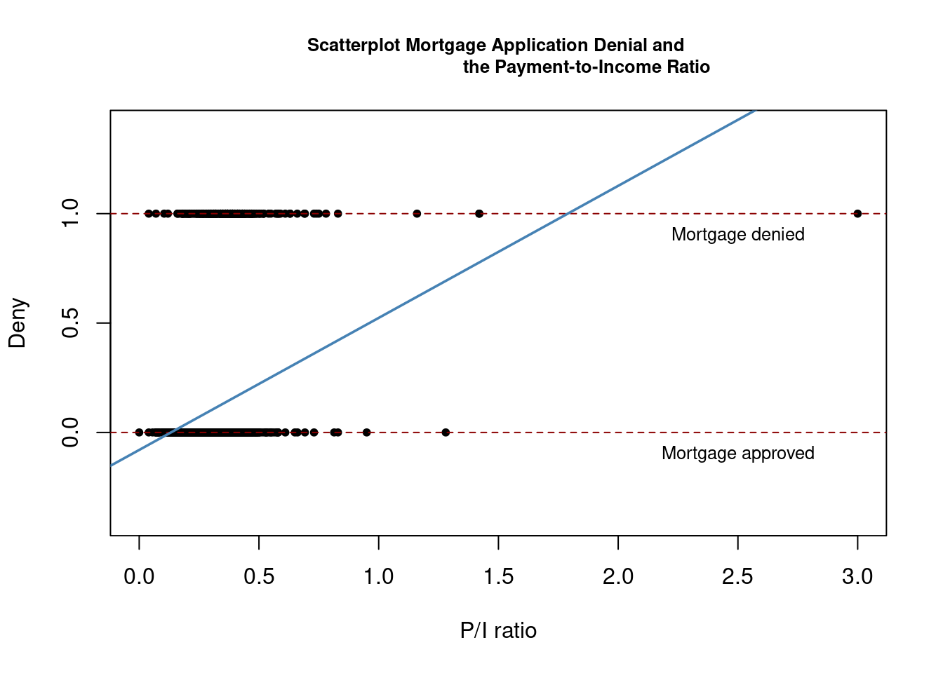
According to the estimated model, a payment-to-income ratio of 1 is associated with an expected probability of mortgage application denial of roughly 50\%.
The model indicates that there is a positive relation between the payment-to-income ratio and the probability of a denied mortgage application. This suggests that individuals with a high ratio of loan payments to income are associated with a higher chance of being rejected.
We may use coeftest() to obtain robust standard errors for both coefficient estimates.
# print robust coefficient summary
coeftest(denymod1, vcov. = vcovHC, type = "HC1")
t test of coefficients:

             Estimate Std. Error t value  Pr(>|t|)
(Intercept) -0.079910   0.031967 -2.4998   0.01249 *
pirat        0.603535   0.098483  6.1283 1.036e-09 ***
---
Signif. codes:  0 '***' 0.001 '**' 0.01 '*' 0.05 '.' 0.1 ' ' 1
The estimated regression line is
\widehat{deny} = \underset{(0.032)}{-0.080} + \underset{(0.098)}{0.604} \, P/I \, ratio \tag{4.2}
The coefficient on P/I \, ratio is statistically different from 0 at the 0.1\% level. Its estimate can be interpreted as follows: a 1 percentage point increase in P/I \, ratio is associated with an average increase in the probability of a loan denial by 0.604 \cdot 0.01 = 0.00604 \approx 0.6 percentage points.
3.3 Is there Racial Discrimination in the Mortgage Market?
We will now augment the simple model (4.2) by adding an additional regressor: black, which equals 1 if the applicant is African American and equals 0 otherwise.
Such a specification is the baseline for investigating if there is racial discrimination in the mortgage market: if being black has a significant (positive) influence on the probability of a loan denial when we control for factors that allow for an objective assessment of an applicant’s creditworthiness, this could be an indicator for discrimination.
In this data set, the variable afam indicates whether the applicant is an African American or not. We will first rename this variable to black for consistency and then we will estimate the model including this new regressor.
# rename the variable 'afam'
colnames(HMDA)[colnames(HMDA) == "afam"] <- "black"

# estimate the model
denymod2 <- lm(deny ~ pirat + black, data = HMDA)
coeftest(denymod2, vcov. = vcovHC)
t test of coefficients:

             Estimate Std. Error t value  Pr(>|t|)
(Intercept) -0.090514   0.033430 -2.7076  0.006826 **
pirat        0.559195   0.103671  5.3939 7.575e-08 ***
blackyes     0.177428   0.025055  7.0815 1.871e-12 ***
---
Signif. codes:  0 '***' 0.001 '**' 0.01 '*' 0.05 '.' 0.1 ' ' 1
The estimated regression function is
\widehat{deny} = \underset{(0.033)}{-0.091} + \underset{(0.104)}{0.559} \, P/I \, ratio + \underset{(0.025)}{0.177} \, black \tag{4.3}
The coefficient on black is positive and significantly different from zero at the 0.1\% level. The interpretation is that, holding constant the P/I \, ratio, being black is associated with an average increase in the probability of a mortgage application denial by 17.7 percentage points.
This finding could be associated with racial discrimination. However, it might be distorted by omitted variable bias so discrimination could be a premature conclusion.
3.4 Probit and Logit Regression
The linear probability model has a major flaw: it assumes the conditional probability function to be linear. This does not restrict P(Y=1|X_1, \ldots , X_k) to lie between 0 and 1.
We can easily observe this in our previous plot for model (4.2): for P/I \, ratio = 1.75, the model predicts the probability of a mortgage application denial to be bigger than 1. For applications with P/I \, ratio close to 0, the predicted probability of denial is even negative, so that the model has no meaningful interpretation here.
From this we can infer the need for a nonlinear function to model the conditional probability function of a binary dependent variable. Commonly used methods are Probit and Logit regression.
3.4.1 Probit Regression
Assume that Y is a binary variable. The model
Y = \beta_0 + \beta_1 X_1 + \beta_2 X_2 + \cdots + \beta_k X_k + u
with
P(Y=1|X_1, X_2 \ldots , X_k) = \Phi(\beta_0 + \beta_1 X_1 + \beta_2 X_2 + \cdots + \beta_k X_k) is the population Probit model, with multiple regressors X_1, X_2 \ldots , X_k and \Phi (\cdot) being the cumulative distribution function (CDF) of a standard normal distribution.
The predicted probability that Y=1 given X_1, X_2 \ldots , X_k can be calculated in two steps:
- Compute z = \beta_0 + \beta_1 X_1 + \beta_2 X_2 + \cdots + \beta_k X_k
- Look up \Phi (z) by calling
pnorm()
\beta_j is the effect on z of a one unit change in regressor X_j, holding constant all other k-1 regressors.
The effect on the predicted probability of a change in a regressor can be computed also in two steps:
- Compute the predicted probability of Y=1 for two cases:
- Case 1: Using the original values of the regressors (X_1, X_2, \ldots, X_k).
- Case 2: Using the modified value of X_1 (X_1 + \Delta X_1) while keeping other regressors constant.
- The difference between the predicted probabilities in Case 1 and Case 2 gives the expected change in the predicted probability of Y=1 associated with the change in X_1.
\Delta \hat{Y} = \hat{P}(Y=1|X_1 + \Delta X_1, X_2, \ldots , X_k) - \hat{P}(Y=1|X_1, X_2, \ldots , X_k) Where \hat{P}(Y=1|X_1, X_2, \ldots , X_k) represents the predicted probability of Y=1 based on the estimated probit model.
In R, Probit models can be estimated using the function glm() from the package stats. Using the argument family we specify that we want to use a Probit link function.
We can now estimate a simple Probit model of the probability of a mortgage denial. Since we have a binary dependent variable, we need to set family = binomial and for this case, we will set link = "probit".
# estimate the simple probit model
denyprobit <- glm(deny ~ pirat, family = binomial(link = "probit"), data = HMDA)

coeftest(denyprobit, vcov. = vcovHC, type = "HC1")
z test of coefficients:

            Estimate Std. Error  z value  Pr(>|z|)
(Intercept) -2.19415    0.18901 -11.6087 < 2.2e-16 ***
pirat        2.96787    0.53698   5.5269 3.259e-08 ***
---
Signif. codes:  0 '***' 0.001 '**' 0.01 '*' 0.05 '.' 0.1 ' ' 1
Just as in the linear probability model, we find that the relation between the probability of denial and the payments-to-income ratio is positive and that the corresponding coefficient is highly significant.
The estimated model is
P \widehat{(deny | P/I \, ratio)} = \Phi (\underset{(0.19)}{-2.19} + \underset{(0.54)}{2.97}\, P/I \,ratio) \tag{4.4}
We can plot this probit model with the following code chunk
# plot data
plot(x = HMDA$pirat, y = HMDA$deny,
     main = "Probit Model of the Probability of Denial, Given P/I Ratio",
     xlab = "P/I ratio", ylab = "Deny",
     pch = 20, ylim = c(-0.4, 1.4), cex.main = 0.85)

# add horizontal dashed lines and text
abline(h = 1, lty = 2, col = "darkred")
abline(h = 0, lty = 2, col = "darkred")
text(2.5, 0.9, cex = 0.8, "Mortgage denied")
text(2.5, -0.1, cex= 0.8, "Mortgage approved")

# add estimated regression line
x <- seq(0, 3, 0.01)
y <- predict(denyprobit, list(pirat = x), type = "response")
lines(x, y, lwd = 1.5, col = "steelblue")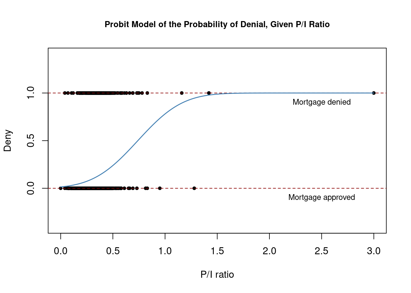
As observed here, the estimated regression function has a “stretched S-shape”. This is typical for the cumulative distribution function of a continuous random variable with symmetric probability density function, like that of a normal random variable.
The function is clearly nonlinear and flattens out for large and small values of P/I \, ratio. The functional form thus ensures that the predicted conditional probabilities of a denial lie between 0 and 1.
How would the denial probability change if we increase the P/I \, ratio from 0.3 to 0.4? We can use predict() and diff() functions to compute the predicted change:
# 1. compute predictions for P/I ratio = 0.3, 0.4
predictions <- predict(denyprobit, newdata = data.frame("pirat" = c(0.3, 0.4)),
                       type = "response")
predictions
1 2
0.09615344 0.15696777 # 2. Compute difference in probabilities
diff(predictions) 2
0.06081433 According to our model, an increase in the P/I \, ratio from 0.3 to 0.4 leads to an average increase in the probability of denial of 6.1 percentage points.
Let’s now include the variable black in our Probit model to further estimate the effect of race on the probability of a mortgage application denial.
# estimate the augmented probit model
denyprobit2 <- glm(deny ~ pirat + black, family = binomial(link = "probit"),
                   data = HMDA)

coeftest(denyprobit2, vcov. = vcovHC, type = "HC1")
z test of coefficients:

             Estimate Std. Error  z value  Pr(>|z|)
(Intercept) -2.258787   0.176608 -12.7898 < 2.2e-16 ***
pirat        2.741779   0.497673   5.5092 3.605e-08 ***
blackyes     0.708155   0.083091   8.5227 < 2.2e-16 ***
---
Signif. codes:  0 '***' 0.001 '**' 0.01 '*' 0.05 '.' 0.1 ' ' 1
The coefficients on P/I , ratio and black appear to be positive and highly significant.
While their interpretation can be sensitive and challenging, this probit model indicates two key findings: first, black applicants, on average, have a higher probability of denial than white applicants, holding the payments-to-income ratio constant; second, applicants with a higher payments-to-income ratio, regardless of their race, face on average a higher risk of rejection.
The estimated model equation is
P \widehat{(deny | P/I \, ratio, black)} = \Phi (\underset{(0.18)}{-2.26} + \underset{(0.50)}{2.74}\, P/I \,ratio + \underset{(0.08)}{0.71} \, black) \tag{4.5}
How big is the estimated difference in denial probabilities between two hypothetical applicants with the same payments-to-income ratio? Just like before, we can compute the difference in probabilities to answer this question according to our estimated model:
# 1. compute predictions with a constant P/I ratio of 0.3
predictions <- predict(denyprobit2,
                       newdata = data.frame("black" = c("no", "yes"),
                                            "pirat" = c(0.3, 0.3)),
                       type = "response")
predictions
1 2
0.07546516 0.23327685 # 2. compute difference in probabilities
diff(predictions) 2
0.1578117 The result indicates that the estimated difference in denial probabilities between a “black” and a “non-black” applicant, both with a payment-to-income ratio of 0.3, is on average 15.8 percentage points higher for the “black” applicant.
3.4.2 Logit regression
The population Logit regression function is
\begin{align*} P(Y = 1 | X_1, X_2, \ldots, X_k) &= F(\beta_0 + \beta_1 X_1 + \beta_2 X_2 + \cdots + \beta_k X_k) \\ &= \frac{1}{1 + e^{-(\beta_0 + \beta_1 X_1 + \beta_2 X_2 + \cdots + \beta_k X_k)}} \end{align*}
The idea is similar to the Probit regression except that here, the probability of the dependent variable Y being 1 given a set of independent variables X_1, X_2, \ldots, X_k is modeled using the cumulative distribution function (CDF) of a standard logistically distributed random variable:
F(x) = \frac{1}{1 + e^{-x}}
As for Probit regression, there is no simple interpretation of the model coefficients and it is best to consider predicted probabilities or differences in predicted probabilities.
The estimation of the Logit regression model in R is again a straightforward process. However, for this specific case, we should specify link = "logit":
denylogit <- glm(deny ~ pirat, family = binomial(link = "logit"), data = HMDA)

coeftest(denylogit, vcov. = vcovHC, type = "HC1")
z test of coefficients:

            Estimate Std. Error  z value  Pr(>|z|)
(Intercept) -4.02843    0.35898 -11.2218 < 2.2e-16 ***
pirat        5.88450    1.00015   5.8836 4.014e-09 ***
---
Signif. codes:  0 '***' 0.001 '**' 0.01 '*' 0.05 '.' 0.1 ' ' 1
The estimated model is
P \widehat{(deny | P/I \, ratio)} = F(\underset{(0.36)}{-4.03} + \underset{(1.00)}{5.88}\, P/I \,ratio ) \tag{4.6}
We can now plot both estimated models to visualize and compare results:
# plot data
plot(x = HMDA$pirat, y = HMDA$deny,
     main = "Probit and Logit Models of the Probability of Denial, Given P/I Ratio",
     xlab = "P/I ratio", ylab = "Deny", pch = 20, ylim = c(-0.4, 1.4), cex.main = 0.9)

# add horizontal dashed lines and text
abline(h = 1, lty = 2, col = "darkred")
abline(h = 0, lty = 2, col = "darkred")
text(2.5, 0.9, cex = 0.8, "Mortgage denied")
text(2.5, -0.1, cex= 0.8, "Mortgage approved")

# add estimated regression line of Probit and Logit models
x <- seq(0, 3, 0.01)
y_probit <- predict(denyprobit, list(pirat = x), type = "response")
y_logit <- predict(denylogit, list(pirat = x), type = "response")
lines(x, y_probit, lwd = 1.5, col = "steelblue")
lines(x, y_logit, lwd = 1.5, col = "black", lty = 2)

# add a legend
legend("topleft",horiz = TRUE, legend = c("Probit", "Logit"),
       col = c("steelblue", "black"), lty = c(1, 2))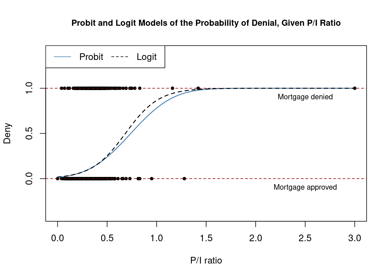
Both models produce very similar estimates of the probability of a mortgage application being denied based on the applicants’ payment-to-income ratio.
Now we may also extend the Logit model by including the variable black
# estimate a Logit regression with multiple regressors
denylogit2 <- glm(deny ~ pirat + black, family = binomial(link = "logit"),
                  data = HMDA)

coeftest(denylogit2, vcov. = vcovHC, type = "HC1")
z test of coefficients:

            Estimate Std. Error  z value  Pr(>|z|)
(Intercept) -4.12556    0.34597 -11.9245 < 2.2e-16 ***
pirat        5.37036    0.96376   5.5723 2.514e-08 ***
blackyes     1.27278    0.14616   8.7081 < 2.2e-16 ***
---
Signif. codes:  0 '***' 0.001 '**' 0.01 '*' 0.05 '.' 0.1 ' ' 1
We obtain
P \widehat{(deny | P/I \, ratio, black)} = F (\underset{(0.35)}{-4.13} + \underset{(0.96)}{5.37}\, P/I \,ratio + \underset{(0.15)}{1.27} \, black) \tag{4.7}
As for the Probit model (4.6) all model coefficients are highly significant and we obtain positive estimates for the coefficients on P/I ratio and black.
For comparison we compute the predicted probability of denial for two hypothetical applicants that differ in race and have a P/I ratio of 0.3.
# 1. compute predictions for P/I ratio = 0.3
predictions <- predict(denylogit2,
                       newdata = data.frame("black" = c("no", "yes"),
                                            "pirat" = c(0.3, 0.3)),
                       type = "response")

predictions
1 2
0.07485143 0.22414592 # 2. Compute difference in probabilities
diff(predictions) 2
0.1492945 We find that, according to our model, white applicants with a payment-to-income of 0.3 face on average a denial probability of only 7.5\%, while African Americans with the same payment-to-income are rejected on average with a probability of 22.4\%, which is 14.9 percentage points higher.
3.5 Comparison of the models
The Probit and the Logit models deliver only approximations to the unknown population regression function E(Y|X). It is not obvious how to decide which model to use in practice.
The linear probability model has the clear drawback of not being able to capture the nonlinear nature of the population regression function and it may predict probabilities to lie outside the interval [0,1].
Probit and Logit models are harder to interpret but they capture the nonlinearities better than the linear approach: both models produce predictions of probabilities that lie inside the interval [0,1]. Predictions of all three models are often close to each other.
The best choice usually depends on the specific characteristics of the data, the theory behind the model relative to the case being studied, and practical considerations like interpretability and the preferences of the audience for the analysis.
It is often suggested to use the method that is easiest to use in the statistical software of choice. As we have seen, it is equally easy to estimate Probit and Logit model using R. The choice between them might come down to other considerations such as the specific distributional assumptions behind each model (Logit assumes a logistic distribution of the error terms, while Probit assumes a normal distribution), the context of the analysis, or the preferences of the analyst. There is therefore no general recommendation for which method to use.
3.6 Controlling for applicant characteristics & financial variables
Models (11.6) and (11.7) indicate that denial rates are higher for African American applicants holding constant the payment-to-income ratio. Both results could be subject to omitted variable bias.
In order to obtain a more trustworthy estimate of the effect of being black on the probability of a mortgage application denial we estimate a linear probability model as well as several Logit and Probit models, but this time we control for financial variables and additional applicant characteristics which are likely to influence the probability of denial and differ between black and white applicants:
-
hirat: inhouse expense-to-total-income ratio. -
lvrat: loan-to-value ratio -
chist: consumer credit score -
mhist: mortgage credit score -
phist: public bad credit record -
insurance: denied mortgage insurance (factor) -
selfemp: self-employed (factor) -
single: single (factor) -
hschool: high school diploma (factor) -
unemp: unemployment rate -
condomin: condominium (factor)
For more on variables contained in the HMDA data set use R’s help() function.
Sample averages can be easily reproduced using the functions mean() (as usual for numeric variables) and prop.table() (for factor variables). For example:
# inhouse expense-to-total-income ratio
mean(HMDA$hirat)
[1] 0.2553461# self-employed
prop.table(table(HMDA$selfemp))
       no       yes
0.8836134 0.1163866
Before estimating the models we transform the loan-to-value ratio (lvrat) into a factor variable, where
lvrat = \begin{cases} \text{low} & \text{if } lvrat < 0.8 \\ \text{medium} & \text{if } 0.8 \leq lvrat \leq 0.95 \\ \text{high} & \text{if } lvrat > 0.95 \end{cases}
and convert both credit scores to numeric variables.
# define low, medium and high loan-to-value ratio
HMDA$lvrat <- factor(
  ifelse(HMDA$lvrat < 0.8, "low",
  ifelse(HMDA$lvrat >= 0.8 & HMDA$lvrat <= 0.95, "medium", "high")),
  levels = c("low", "medium", "high"))

# convert credit scores to numeric
HMDA$mhist <- as.numeric(HMDA$mhist)
HMDA$chist <- as.numeric(HMDA$chist)
Next, we estimate different models for denial probability
# estimate 6 models for the denial probability
lpm <- lm(deny ~ black + pirat + hirat + lvrat + chist + mhist + phist
               + insurance + selfemp, data = HMDA)

logit <- glm(deny ~ black + pirat + hirat + lvrat + chist + mhist + phist
                  + insurance + selfemp,
                  family = binomial(link = "logit"),
                  data = HMDA)

probit1 <- glm(deny ~ black + pirat + hirat + lvrat + chist + mhist + phist
                     + insurance + selfemp,
                     family = binomial(link = "probit"),
                     data = HMDA)

probit2 <- glm(deny ~ black + pirat + hirat + lvrat + chist + mhist + phist
                     + insurance + selfemp + single + hschool + unemp,
                     family = binomial(link = "probit"),
                     data = HMDA)

probit3 <- glm(deny ~ black + pirat + hirat + lvrat + chist + mhist
                     + phist + insurance + selfemp + single + hschool + unemp
                     +condomin + I(mhist==3) + I(mhist==4) + I(chist==3)
                     + I(chist==4) + I(chist==5)+ I(chist==6),
                     family = binomial(link = "probit"), data = HMDA)

probit4 <- glm(deny ~ black * (pirat + hirat) + lvrat + chist + mhist + phist
                     + insurance + selfemp + single + hschool + unemp,
                     family = binomial(link = "probit"), data = HMDA)
Then we store heteroskedasticity-robust standard errors of the coefficient estimators in a list which is then used as the argument se in stargazer()
rob_se <- list(sqrt(diag(vcovHC(lpm, type = "HC1"))),
               sqrt(diag(vcovHC(logit, type = "HC1"))),
               sqrt(diag(vcovHC(probit1, type = "HC1"))),
               sqrt(diag(vcovHC(probit2, type = "HC1"))),
               sqrt(diag(vcovHC(probit3, type = "HC1"))),
               sqrt(diag(vcovHC(probit4, type = "HC1"))))

stargazer(lpm, logit, probit1, probit2, probit3, probit4,
          se = rob_se,
          type="html",
          omit.stat = "f", df=FALSE)
<table style="text-align:center"><tr><td colspan="7" style="border-bottom: 1px solid black"></td></tr><tr><td style="text-align:left"></td><td colspan="6"><em>Dependent variable:</em></td></tr>
<tr><td></td><td colspan="6" style="border-bottom: 1px solid black"></td></tr>
<tr><td style="text-align:left"></td><td colspan="6">deny</td></tr>
<tr><td style="text-align:left"></td><td><em>OLS</em></td><td><em>logistic</em></td><td colspan="4"><em>probit</em></td></tr>
<tr><td style="text-align:left"></td><td>(1)</td><td>(2)</td><td>(3)</td><td>(4)</td><td>(5)</td><td>(6)</td></tr>
<tr><td colspan="7" style="border-bottom: 1px solid black"></td></tr><tr><td style="text-align:left">blackyes</td><td>0.084<sup>***</sup></td><td>0.688<sup>***</sup></td><td>0.389<sup>***</sup></td><td>0.371<sup>***</sup></td><td>0.363<sup>***</sup></td><td>0.246</td></tr>
<tr><td style="text-align:left"></td><td>(0.023)</td><td>(0.183)</td><td>(0.099)</td><td>(0.100)</td><td>(0.101)</td><td>(0.479)</td></tr>
<tr><td style="text-align:left"></td><td></td><td></td><td></td><td></td><td></td><td></td></tr>
<tr><td style="text-align:left">pirat</td><td>0.449<sup>***</sup></td><td>4.764<sup>***</sup></td><td>2.442<sup>***</sup></td><td>2.464<sup>***</sup></td><td>2.622<sup>***</sup></td><td>2.572<sup>***</sup></td></tr>
<tr><td style="text-align:left"></td><td>(0.114)</td><td>(1.332)</td><td>(0.673)</td><td>(0.654)</td><td>(0.665)</td><td>(0.728)</td></tr>
<tr><td style="text-align:left"></td><td></td><td></td><td></td><td></td><td></td><td></td></tr>
<tr><td style="text-align:left">hirat</td><td>-0.048</td><td>-0.109</td><td>-0.185</td><td>-0.302</td><td>-0.502</td><td>-0.538</td></tr>
<tr><td style="text-align:left"></td><td>(0.110)</td><td>(1.298)</td><td>(0.689)</td><td>(0.689)</td><td>(0.715)</td><td>(0.755)</td></tr>
<tr><td style="text-align:left"></td><td></td><td></td><td></td><td></td><td></td><td></td></tr>
<tr><td style="text-align:left">lvratmedium</td><td>0.031<sup>**</sup></td><td>0.464<sup>***</sup></td><td>0.214<sup>***</sup></td><td>0.216<sup>***</sup></td><td>0.215<sup>**</sup></td><td>0.216<sup>***</sup></td></tr>
<tr><td style="text-align:left"></td><td>(0.013)</td><td>(0.160)</td><td>(0.082)</td><td>(0.082)</td><td>(0.084)</td><td>(0.083)</td></tr>
<tr><td style="text-align:left"></td><td></td><td></td><td></td><td></td><td></td><td></td></tr>
<tr><td style="text-align:left">lvrathigh</td><td>0.189<sup>***</sup></td><td>1.495<sup>***</sup></td><td>0.791<sup>***</sup></td><td>0.795<sup>***</sup></td><td>0.836<sup>***</sup></td><td>0.788<sup>***</sup></td></tr>
<tr><td style="text-align:left"></td><td>(0.050)</td><td>(0.325)</td><td>(0.183)</td><td>(0.184)</td><td>(0.185)</td><td>(0.185)</td></tr>
<tr><td style="text-align:left"></td><td></td><td></td><td></td><td></td><td></td><td></td></tr>
<tr><td style="text-align:left">chist</td><td>0.031<sup>***</sup></td><td>0.290<sup>***</sup></td><td>0.155<sup>***</sup></td><td>0.158<sup>***</sup></td><td>0.344<sup>***</sup></td><td>0.158<sup>***</sup></td></tr>
<tr><td style="text-align:left"></td><td>(0.005)</td><td>(0.039)</td><td>(0.021)</td><td>(0.021)</td><td>(0.108)</td><td>(0.021)</td></tr>
<tr><td style="text-align:left"></td><td></td><td></td><td></td><td></td><td></td><td></td></tr>
<tr><td style="text-align:left">mhist</td><td>0.021<sup>*</sup></td><td>0.279<sup>**</sup></td><td>0.148<sup>**</sup></td><td>0.110</td><td>0.162</td><td>0.111</td></tr>
<tr><td style="text-align:left"></td><td>(0.011)</td><td>(0.138)</td><td>(0.073)</td><td>(0.076)</td><td>(0.104)</td><td>(0.077)</td></tr>
<tr><td style="text-align:left"></td><td></td><td></td><td></td><td></td><td></td><td></td></tr>
<tr><td style="text-align:left">phistyes</td><td>0.197<sup>***</sup></td><td>1.226<sup>***</sup></td><td>0.697<sup>***</sup></td><td>0.702<sup>***</sup></td><td>0.717<sup>***</sup></td><td>0.705<sup>***</sup></td></tr>
<tr><td style="text-align:left"></td><td>(0.035)</td><td>(0.203)</td><td>(0.114)</td><td>(0.115)</td><td>(0.116)</td><td>(0.115)</td></tr>
<tr><td style="text-align:left"></td><td></td><td></td><td></td><td></td><td></td><td></td></tr>
<tr><td style="text-align:left">insuranceyes</td><td>0.702<sup>***</sup></td><td>4.548<sup>***</sup></td><td>2.557<sup>***</sup></td><td>2.585<sup>***</sup></td><td>2.589<sup>***</sup></td><td>2.590<sup>***</sup></td></tr>
<tr><td style="text-align:left"></td><td>(0.045)</td><td>(0.576)</td><td>(0.305)</td><td>(0.299)</td><td>(0.306)</td><td>(0.299)</td></tr>
<tr><td style="text-align:left"></td><td></td><td></td><td></td><td></td><td></td><td></td></tr>
<tr><td style="text-align:left">selfempyes</td><td>0.060<sup>***</sup></td><td>0.666<sup>***</sup></td><td>0.359<sup>***</sup></td><td>0.346<sup>***</sup></td><td>0.342<sup>***</sup></td><td>0.348<sup>***</sup></td></tr>
<tr><td style="text-align:left"></td><td>(0.021)</td><td>(0.214)</td><td>(0.113)</td><td>(0.116)</td><td>(0.116)</td><td>(0.116)</td></tr>
<tr><td style="text-align:left"></td><td></td><td></td><td></td><td></td><td></td><td></td></tr>
<tr><td style="text-align:left">singleyes</td><td></td><td></td><td></td><td>0.229<sup>***</sup></td><td>0.230<sup>***</sup></td><td>0.226<sup>***</sup></td></tr>
<tr><td style="text-align:left"></td><td></td><td></td><td></td><td>(0.080)</td><td>(0.086)</td><td>(0.081)</td></tr>
<tr><td style="text-align:left"></td><td></td><td></td><td></td><td></td><td></td><td></td></tr>
<tr><td style="text-align:left">hschoolyes</td><td></td><td></td><td></td><td>-0.613<sup>***</sup></td><td>-0.604<sup>**</sup></td><td>-0.620<sup>***</sup></td></tr>
<tr><td style="text-align:left"></td><td></td><td></td><td></td><td>(0.229)</td><td>(0.237)</td><td>(0.229)</td></tr>
<tr><td style="text-align:left"></td><td></td><td></td><td></td><td></td><td></td><td></td></tr>
<tr><td style="text-align:left">unemp</td><td></td><td></td><td></td><td>0.030<sup>*</sup></td><td>0.028</td><td>0.030</td></tr>
<tr><td style="text-align:left"></td><td></td><td></td><td></td><td>(0.018)</td><td>(0.018)</td><td>(0.018)</td></tr>
<tr><td style="text-align:left"></td><td></td><td></td><td></td><td></td><td></td><td></td></tr>
<tr><td style="text-align:left">condominyes</td><td></td><td></td><td></td><td></td><td>-0.055</td><td></td></tr>
<tr><td style="text-align:left"></td><td></td><td></td><td></td><td></td><td>(0.096)</td><td></td></tr>
<tr><td style="text-align:left"></td><td></td><td></td><td></td><td></td><td></td><td></td></tr>
<tr><td style="text-align:left">I(mhist == 3)</td><td></td><td></td><td></td><td></td><td>-0.107</td><td></td></tr>
<tr><td style="text-align:left"></td><td></td><td></td><td></td><td></td><td>(0.301)</td><td></td></tr>
<tr><td style="text-align:left"></td><td></td><td></td><td></td><td></td><td></td><td></td></tr>
<tr><td style="text-align:left">I(mhist == 4)</td><td></td><td></td><td></td><td></td><td>-0.383</td><td></td></tr>
<tr><td style="text-align:left"></td><td></td><td></td><td></td><td></td><td>(0.427)</td><td></td></tr>
<tr><td style="text-align:left"></td><td></td><td></td><td></td><td></td><td></td><td></td></tr>
<tr><td style="text-align:left">I(chist == 3)</td><td></td><td></td><td></td><td></td><td>-0.226</td><td></td></tr>
<tr><td style="text-align:left"></td><td></td><td></td><td></td><td></td><td>(0.248)</td><td></td></tr>
<tr><td style="text-align:left"></td><td></td><td></td><td></td><td></td><td></td><td></td></tr>
<tr><td style="text-align:left">I(chist == 4)</td><td></td><td></td><td></td><td></td><td>-0.251</td><td></td></tr>
<tr><td style="text-align:left"></td><td></td><td></td><td></td><td></td><td>(0.338)</td><td></td></tr>
<tr><td style="text-align:left"></td><td></td><td></td><td></td><td></td><td></td><td></td></tr>
<tr><td style="text-align:left">I(chist == 5)</td><td></td><td></td><td></td><td></td><td>-0.789<sup>*</sup></td><td></td></tr>
<tr><td style="text-align:left"></td><td></td><td></td><td></td><td></td><td>(0.412)</td><td></td></tr>
<tr><td style="text-align:left"></td><td></td><td></td><td></td><td></td><td></td><td></td></tr>
<tr><td style="text-align:left">I(chist == 6)</td><td></td><td></td><td></td><td></td><td>-0.905<sup>*</sup></td><td></td></tr>
<tr><td style="text-align:left"></td><td></td><td></td><td></td><td></td><td>(0.515)</td><td></td></tr>
<tr><td style="text-align:left"></td><td></td><td></td><td></td><td></td><td></td><td></td></tr>
<tr><td style="text-align:left">blackyes:pirat</td><td></td><td></td><td></td><td></td><td></td><td>-0.579</td></tr>
<tr><td style="text-align:left"></td><td></td><td></td><td></td><td></td><td></td><td>(1.550)</td></tr>
<tr><td style="text-align:left"></td><td></td><td></td><td></td><td></td><td></td><td></td></tr>
<tr><td style="text-align:left">blackyes:hirat</td><td></td><td></td><td></td><td></td><td></td><td>1.232</td></tr>
<tr><td style="text-align:left"></td><td></td><td></td><td></td><td></td><td></td><td>(1.709)</td></tr>
<tr><td style="text-align:left"></td><td></td><td></td><td></td><td></td><td></td><td></td></tr>
<tr><td style="text-align:left">Constant</td><td>-0.183<sup>***</sup></td><td>-5.707<sup>***</sup></td><td>-3.041<sup>***</sup></td><td>-2.575<sup>***</sup></td><td>-2.896<sup>***</sup></td><td>-2.543<sup>***</sup></td></tr>
<tr><td style="text-align:left"></td><td>(0.028)</td><td>(0.484)</td><td>(0.250)</td><td>(0.350)</td><td>(0.404)</td><td>(0.370)</td></tr>
<tr><td style="text-align:left"></td><td></td><td></td><td></td><td></td><td></td><td></td></tr>
<tr><td colspan="7" style="border-bottom: 1px solid black"></td></tr><tr><td style="text-align:left">Observations</td><td>2,380</td><td>2,380</td><td>2,380</td><td>2,380</td><td>2,380</td><td>2,380</td></tr>
<tr><td style="text-align:left">R<sup>2</sup></td><td>0.266</td><td></td><td></td><td></td><td></td><td></td></tr>
<tr><td style="text-align:left">Adjusted R<sup>2</sup></td><td>0.263</td><td></td><td></td><td></td><td></td><td></td></tr>
<tr><td style="text-align:left">Log Likelihood</td><td></td><td>-635.637</td><td>-636.847</td><td>-628.614</td><td>-625.064</td><td>-628.332</td></tr>
<tr><td style="text-align:left">Akaike Inf. Crit.</td><td></td><td>1,293.273</td><td>1,295.694</td><td>1,285.227</td><td>1,292.129</td><td>1,288.664</td></tr>
<tr><td style="text-align:left">Residual Std. Error</td><td>0.279</td><td></td><td></td><td></td><td></td><td></td></tr>
<tr><td colspan="7" style="border-bottom: 1px solid black"></td></tr><tr><td style="text-align:left"><em>Note:</em></td><td colspan="6" style="text-align:right"><sup>*</sup>p<0.1; <sup>**</sup>p<0.05; <sup>***</sup>p<0.01</td></tr>
</table>
Models (1), (2) and (3) are baseline specifications that include several financial control variables. They differ only in the way they model the denial probability. Model (1) is a linear probability model, model (2) is a Logit regression and model (3) uses the Probit approach.
In the linear model (1), the coefficients have direct interpretation. For example:
An increase in the consumer credit score by 1 unit is estimated to increase the probability of a loan denial on average by 3.1 percentage points.
Having a high loan-to-value ratio is detriment for credit approval: the coefficient for a loan-to-value ratio higher than 0.95 is 0.189 so clients with this property are estimated to face an almost 19 percentage points larger risk of denial on average than those with a low loan-to-value ratio, ceteris paribus.
The estimated coefficient on the race dummy is 0.084, which indicates the denial probability for African Americans is estimated to be on average 8.4 percentage points larger than for white applicants with the same characteristics except for race.
Apart from the inhouse expense-to-total-income ratio, all coefficients are significant in the linear probability model.
Models (2) and (3) provide similar evidence of racial discrimination in the U.S. mortgage market. All coefficients except for the housing expense-to-income ratio (which is not significantly different from zero) and the mortgage credit score (which is statistically significant at the 5\% level) are significant at the 1\% level.
As discussed above, the nonlinearity makes the interpretation of the coefficient estimates more difficult than for model (1).
In order to make a statement about the effect of being black, we need to compute the estimated denial probability for two individuals that differ only in race. For the comparison we consider two individuals that share mean values for all numeric regressors.
For the qualitative variables we assign the property that is most representative for the data at hand. For example, consider self-employment: we have seen that about 88\% of all individuals in the sample are not self-employed such that we set selfemp = no.
Using this approach, the estimate for the effect on the denial probability of being African American according to the Logit model (2) would be 4 percentage points. The next code chunk shows how to apply this approach for models (1) to (6) using R.
# compute regressor values for an average black person
new <- data.frame(
  "pirat" = mean(HMDA$pirat),
  "hirat" = mean(HMDA$hirat),
  "lvrat" = "low",
  "chist" = mean(HMDA$chist),
  "mhist" = mean(HMDA$mhist),
  "phist" = "no",
  "insurance" = "no",
  "selfemp" = "no",
  "black" = c("no", "yes"),
  "single" = "no",
  "hschool" = "yes",
  "unemp" = mean(HMDA$unemp),
  "condomin" = "no")

# difference predicted by the LPM (1)
predictions <- predict(lpm, newdata = new)
diff(predictions)
2
0.08369674 # difference predicted by the logit model (2)
predictions <- predict(logit, newdata = new, type = "response")
diff(predictions) 2
0.04042135 # difference predicted by probit model (3)
predictions <- predict(probit1, newdata = new, type = "response")
diff(predictions) 2
0.05049716 # difference predicted by probit model (4)
predictions <- predict(probit2, newdata = new, type = "response")
diff(predictions) 2
0.03978918 # difference predicted by probit model (5)
predictions <- predict(probit3, newdata = new, type = "response")
diff(predictions) 2
0.04972468 # difference predicted by probit model (6)
predictions <- predict(probit4, newdata = new, type = "response")
diff(predictions) 2
0.03955893 The estimates of the impact on the denial probability of being black are similar for models (2) and (3). It is interesting that the magnitude of the estimated effects is much smaller than for Probit and Logit models that do not control for financial characteristics (see models 4.5 and 4.7). This indicates that these simple models produced biased estimates due to omitted variables.
Regressions (4) to (6) include different applicant characteristics and credit rating indicator variables, as well as interactions. However, most of the corresponding coefficients are not significant and the estimates of the coefficient on black obtained for these models, as well as the estimated difference in denial probabilities, do not differ much from those obtained for models (2) and (3).
An interesting question related to racial discrimination can be investigated using the Probit model (6) where the interactions blackyes:pirat and blackyes:hirat are added to model (4).
If the coefficient on blackyes:pirat was significantly different from zero, the effect of the payment-to-income ratio on the denial probability would be different for black and white applicants.
Similarly, a non-zero coefficient on blackyes:hirat would indicate that loan officers weight the risk of bankruptcy associated with a high loan-to-value ratio differently for black and white mortgage applicants. We can test whether these coefficients are jointly significant at the 5\% level using an F-Test.
linearHypothesis(probit4,
                 test = "F",
                 c("blackyes:pirat=0", "blackyes:hirat=0"),
                 vcov = vcovHC, type = "HC1")
Linear hypothesis test
Hypothesis:
blackyes:pirat = 0
blackyes:hirat = 0
Model 1: restricted model
Model 2: deny ~ black * (pirat + hirat) + lvrat + chist + mhist + phist +
insurance + selfemp + single + hschool + unemp
Note: Coefficient covariance matrix supplied.
Res.Df Df F Pr(>F)
1 2366
2 2364 2 0.2473 0.7809Since p\text{-value} \approx 0.78 for this test, the null cannot be rejected. There is not enough evidence to conclude that there is a significant interaction effect between being black and the variables pirat and hirat when considering the denial outcome.
Nonetheless, when we test whether the coefficients for the main effect of blackyes and the interaction terms blackyes:pirat and blackyes:hirat are jointly equal to zero at the 5\% level, we obtain:
linearHypothesis(probit4, test = "F",
                 c("blackyes=0", "blackyes:pirat=0", "blackyes:hirat=0"),
                 vcov = vcovHC, type = "HC1")
Linear hypothesis test
Hypothesis:
blackyes = 0
blackyes:pirat = 0
blackyes:hirat = 0
Model 1: restricted model
Model 2: deny ~ black * (pirat + hirat) + lvrat + chist + mhist + phist +
insurance + selfemp + single + hschool + unemp
Note: Coefficient covariance matrix supplied.
Res.Df Df F Pr(>F)
1 2367
2 2364 3 4.7774 0.002534 **
---
Signif. codes: 0 '***' 0.001 '**' 0.01 '*' 0.05 '.' 0.1 ' ' 1With p\text{-value} \approx 0.003 we can reject the hypothesis that there is no racial discrimination in the model. There is significant evidence to suggest that at least one of the coefficients for the main effect of blackyes or the interaction terms involving blackyes is not equal to zero.
This suggests the presence of racial discrimination in the model, as the inclusion of blackyes in addition to the interaction terms leads to a significant difference in the model fit.
3.7 Summary
Models (1) to (6) provide evidence that there is an effect of being African American on the probability of mortgage application denial.
In specifications (2) to (5), the effect is estimated to be positive (ranging from 4 to 5 percentage points) and statistically significant at the 1\% level.
While the linear probability model (1) seems to slightly overestimate this positive effect at 8 percentage points, it still can be used as an approximation to an intrinsically nonlinear relationship.
Probit model (6) delved deeper, revealing the presence of racial discrimination through interaction effects between being African American and other variables.