8 Regression Analysis
8.1 Data Collection
Many datasets provided via the WWW:
- Excel/CSV files provided by some organisation (Bundesbank, EZB, Statistisches Bundesamt, Eurostat …)
- Application programming interface (API): Fred Database
- Data scraping (extract data from a HTML code using R or Python)
CSV (Comma-separated values) is the most common format
Checking data for missing values and errors
Tidy data format (variables in columns, obs. in rows)
Compute descriptive statistics (mean, std.dev, min/max, distribution)
Report sufficient info on the data source (for replication)
8.2 Data Preparation
Assess the quality of the data source
Transform text into numerical values (dummy variables)
Plausibility checks / descriptive statistics
data set may contain missing values (‘NA’, dots, blank)
few NA: just ignore them (the row will be dropped)
when many observations lost: imputation (replace NA by estimated values)
a) Multiple Imputation: Assume that x_{k,t} is missing. For available observations run the regression
x_{k,t} = \gamma_0 + \sum_{j=1}^{k-1} \gamma_j x_{j,t} + \epsilon_i \Rightarrow replace the missing values by \hat{x}_{k,t}.
For missing values in more regressors: iterative approach
MaxLike approach available for efficient imputation
8.3 OLS estimator
OLS: Ordinary least-square estimator
b = \underset{\beta}{\text{argmin}} \left\{ (y - X\beta)^\prime (y - X\beta) \right\}yields the least-squares estimator:
b = \color{red} {(X^\prime X)^{-1} X^\prime y}
Unbiased estimator for \sigma^2: (note that X' e = 0)
s^2 = \frac{1}{N - K} (y - Xb)^\prime (y - Xb)
Maximum-Likelihood (ML) estimator
Log-likelihood function assuming normal distribution:
\begin{align*} \ell(\beta, \sigma^2) &= \ln L(\beta, \sigma^2) = \ln \left[ \prod_{i=1}^{N} f(u_i) \right] \\ &= -\frac{N}{2} \ln 2\pi -\frac{N}{2} \ln \sigma^2 - \frac{1}{2\sigma^2} \color{blue}{(y - X\beta)^\prime (y - X\beta)} \end{align*}
ML and OLS of \beta are identical under normality
ML estimator for \sigma^2:
\tilde{\sigma}^2 = \frac{1}{N} (y - Xb)^\prime (y - Xb)
Goodness of fit:
\color{blue}{R^2} \color{black}{ = \frac{ESS}{TSS} = 1 - \frac{SSR}{TSS} =} \quad \color{blue}{1 - \frac{e^\prime e}{y^\prime y - N\bar{y}^2}} \quad \color{black}{=} \quad \color{red}{r^2_{xy}}
adjusted R^2:
\bar{R}^2 = 1 - \frac{e^\prime e/(N - K)} {(y^\prime y - N\bar{y}^2)/(N - 1)}
8.4 Properties of the OLS estimator
a) Expectation \quad [note that b = \color{red}{\beta} \color{black}{+ \underbrace{(X'X)^{-1}X'u}_{\color{blue}{\text{estimation error}}}}]
\begin{align*} & \color{blue}{E(b) = \beta} & \\ & E(s^2) = \sigma^2 & \\ & E(\tilde{\sigma}^2) = \sigma^2 (N - K)/N & \end{align*}
b) Distribution \quad assuming u \sim \mathcal{N}(0, \sigma^2 I_N)
\color{blue}{b \sim \mathcal{N}(\beta, \Sigma_b)}\color{black}{, \quad \Sigma_b = \sigma^2 (X'X)^{-1}}
\frac{(N-K)}{\sigma^2}s^2 \sim \chi^2_{N-K}
c) Efficiency
b is BLUE
under normality: b and s^2 are MVUE
8.5 Testing Hypotheses
Significance level or size of a test (Type I error)
P(|t_k| \geq c_{\alpha/2} | \color{red}{\beta = \beta_0}\color{black}{) = \alpha^*}
where \color{red}{\alpha} is the nominal: size and \color{blue}{\alpha^*} is the actual size
a test is unbiased (controls the size) if \alpha^* = \alpha
a test is asymptotically valid if \alpha^* \rightarrow \alpha for N \rightarrow \infty
1 - type II error or power of the test:
P(|t_k| \geq c_{\alpha/2} | \color{red}{\beta = \beta^1}\color{black}{) = \pi(\beta^1)}
a test is consistent if
\pi(\beta^1) \rightarrow 1 \quad \text{for all} \quad \beta^1 \neq \beta_0
The conventional significance level is \color{red}{\alpha = 0.05} for a moderate sample size (N \in [50, 500], say)
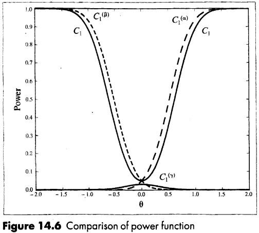
a test is uniform most powerful (UMP) if \color{red}{\pi(\beta) \geq \pi^*(\beta)} \quad \color{black}{\text{for all} \quad \beta \neq \beta^0} where \pi^*(\beta) denotes the power function of any other unbiased test statistic.
\Rightarrow The one-sided t-test is UMP but in many cases there does not exist a UMP test.
The p-value (or marginal significance level) is defined as
\text{p-value} = P(t_k \geq \bar{t}_k | \beta = \beta^0) = 1 - F_0(t_k)
that is, the probability to observe a larger value of the observed statistic \bar{t}_k .
Under the null hypothesis the p-value is uniformly distributed on [0, 1]. Since it is a random variable, it is NOT a probability (that the null hypothesis is correct).
Testing general linear hypotheses on \beta
J linear hypotheses on \beta represented by
H_0 : \quad \color{blue}{R\beta = q}\color{black}{, \quad J \times 1}
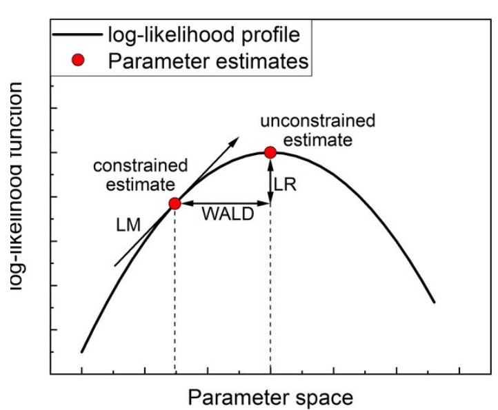
Wald statistic
Rb - q \sim \mathcal{N}\left(0, \sigma^2 R(X'X)^{-1}R' \right)
if \sigma^2 is known:
\frac{1}{\sigma^2} (Rb - q)' [R(X'X)^{-1}R']^{-1} (Rb - q) \sim \chi^2_J
if \sigma^2 is replaces by s^2:
\begin{align*} F &= \frac{1}{Js^2} (Rb - q)' [R(X'X)^{-1}R']^{-1} (Rb - q) = \frac{N - K}{J}\; \color{blue}{\frac{(e_r'e_r - e'e)}{e'e}} \\ &\sim \frac{\chi^2_J/J}{\chi^2_{N-K}/(N - K)} \equiv \color{red}{F^J_{N-K}} \end{align*}
Alternatives to the F statistic
Generalized LR test: GLR = 2 \left( \ell(\hat{\theta}) - \ell(\hat{\theta_r}) \right) = N (\log e'_r e_r - \log e'e) \sim \chi^2_J
\Rightarrow first order Taylor expansion yields the Wald/F statistic
LM (score) test: Define the “’score vector” as: s(\hat{\theta_r}) = \left. \frac{\partial \log L(\theta)}{\partial \theta} \right|_{\theta=\hat{\theta_r}} = \frac{1}{\hat{\sigma}^2_r} X' e_r
The LM test statistic is given by \text{LM} = s(\hat{\theta_r})' I(\hat{\theta_r})^{-1} s(\hat{\theta_r}) \sim \chi^2_J
where I(\hat{\theta_r}) is some estimate of the information matrix
In the regression the LM statistic can be obtained from testing \gamma = 0 the auxiliary regression
1 = \gamma' s_i(\hat{\theta_r}) + \nu_i
\Rightarrow uncentered R^2: R^2_u = \bar{s}' (\sum s_i s'_i)^{-1} \bar{s}. N \cdot R^2_u \sim \chi^2_J
8.5.1 Specification tests
a) Test for Heteroskedasticity (Breusch-Pagan / Koenker)
variance function: \sigma^2_i = \alpha_0 + \color{red}{z'_i \alpha}
since E(\hat{u}^2_i) \approx \sigma^2 estimate the regression \hat{u}^2_i = \alpha_0 + z'_i \alpha + \nu_i \Rightarrow F or LM test statistic for H_0: \color{red}{\alpha = 0}
in practice z_i = x_i but also cross-products and squares of the regressors (White test)
robust (White) standard errors: replace invalid formula Var(b) = \sigma^2(X'X)^{-1} by the estimator: \widehat{Var}(b) = (X'X)^{-1} \left( \sum_{i=1}^{n} \color{red}{\hat{u}^2_i}\color{black}{ x_i x'_i} \right) (X'X)^{-1}
b) Tests for Autocorrelation
(i) Durbin-Watson-Test: dw = \frac{ \sum_{t=2}^{N} (\hat{u}_t - \hat{u}_{t-1})^2}{\sum_{t=1}^{N} \hat{u}^2_t} \approx 2(1 - \color{red}{\hat{\rho}}\color{black}{)} Problem: Distribution depends on X \Rightarrow uncertainty range
(ii) Breusch-Godfrey Test: u_t = \color{blue}{\rho_1 u_{t-1} + \dots + \rho_m u_{t-m}} \color{black}{+ v_t}
replace u_t by \hat{u}_t and include x_t to control for the estimation error in u_t and testing H_0: \color{red}{\rho_1 = \dots = \rho_m = 0}
(iii) Box-Pierce Test: Q_m = T \sum_{j=1}^{m} \color{red}{\hat{\rho}_j}\color{black}{^2 \stackrel{a}{\sim} \chi^2_m} test of autocorrelation up to lag order m
HAC standard errors:
Heteroskedasticity and Autocorrelation Consistent standard errors (Newey/West 1987)
standard errors that account for autocorrelation up to lag h (truncation lag)
“Rule of thumb” for choosing H (e.g. Eviews/Gretl) h = int[4 (T/100)^{2/9}]
Relationship between autocorrelation and dynamic models:
Inserting u_t = \rho u_{t-1} + v_t yields
y_i = \rho y_{t-1} + \beta' x_i - \underbrace{\rho \beta'}_{\gamma} x_{t-1} + v_i \Rightarrow Common factor restriction: \gamma = -\beta\rho
Test for normality
The asymptotic properties of the OLS estimator do not depend on the validity of the normality assumption
Deviations from the normal distribution only relevant in very small samples
Outliers may be modeled by mixing distributions
Tests for normality are very sensitive against outliers
Under the null hypothesis E(u^3_i) = 0 and E(u^4_i) = 3\sigma^4
Jarque-Bera test statistic: JB = n \left[ \color{blue}{\frac{1}{6} \hat{m}_3^2} \color{black}{ + } \color{red}{\frac{1}{24} (\hat{m}_4 - 3)^2\color{black}{} } \right] \stackrel{d}{\to} \chi^2_2
where \hat{m}_3 = \frac{1}{T \hat{\sigma}^3} \sum_{t=1}^{T} \hat{u}^3_i \quad \quad \hat{m}_4 = \frac{1}{T\hat{\sigma}^4} \sum_{t=1}^{T} \hat{u}^4_i
Other tests: \chi^2 and Kolmogorov-Smirnov Test
8.6 Nonlinear regression models
a) Polynomial regression
including squares, cubic etc. transformations of the regressors: Y_i = \beta_0 + \beta_1 X_i + \beta_2 X_i^2 + \dots + \beta_p X_i^p + u_i
where p is the degree of the polynomial (typically p = 2)
Interpretation (for p = 2)
\begin{align*} \frac{\partial Y}{\partial X} &= \beta_1 + 2\beta_2X \\ \Rightarrow \Delta Y &\approx (\beta_1 + 2\beta_2X) \color{red}{\Delta X} \\ \text{exact: } \Delta Y &= \beta_1\Delta X + \beta_2(X + \Delta X)^2 - \beta_2X^2 \\ &= (\beta_1 + 2\beta_2X) \color{red}{\Delta X} \color{black}{+ \beta_2(\Delta X)^2} \end{align*}
\Rightarrow the effect on Y depends on the level of X
for small changes in X the derivative provides a good approximation
Computing standard errors for the nonlinear effect:
Method 1:
\begin{align*} \text{s.e.}\left( \Delta \hat{Y} \right) &= \sqrt{ \text{var}(b_1) + 4X^2 \text{var}(b_2) + 8X \text{cov}(b_1, b_2) } \\ &= |\Delta \hat{Y}| / \sqrt{F} \end{align*}
where F is the F statistic for the test E(\Delta \hat{Y_i}) = \beta_1 + 2X\beta_2 = 0
Method 2:
Y_i = \beta_0 + \underbrace{(\beta_1 + 2X\beta_2)}_{\beta^*_1} X_i + \beta_2 \underbrace{ \left(1 - 2\frac{X}X_i\right)X^2_i}_{X^*_i} + u_i
Regression Y_i = \beta_0 + \beta^*_1 X_i + \beta^*_2 X^*_i + u_i and t-test of \beta^*_1 = 0
Confidence interval for the effect are obtained as \Delta \hat{Y} \pm z_{\alpha/2} \cdot s.e.(\Delta \hat{Y}) or b^*_1 \pm \text{s.e.}(b^*_1)
Logarithmic transformation
Three possible specifications:
\begin{align*} \text{log-linear: } & & \color{blue}{\log} \color{black}{(Y_i)} & = \beta_0 + \beta_1X_i + u_i \\ \text{linear-log: } & & Y_i & = \beta_0 + \beta_1\color{blue}{\log} \color{black}{(X_i)} + u_i \\ \text{log-log: } & & \color{blue}{\log}\color{black}{(Y_i)} & = \beta_0 + \beta_1\color{blue}{\log}\color{black}{(X_i)} + u_i \end{align*}
Note that in the log-linear model
\beta_1 = \frac{d \log(Y)}{d X} = \underbrace{\frac{1}{Y}}_{outer} \cdot \underbrace{\frac{d Y}{d X}}_{inner} = \frac{d Y/Y}{d X} where dY/Y indicates the relative change
In a similar manner it can be shown that for the log-log model \beta_1 = (dY/Y)/(dX/X) is the elasticity
Note that the derivative refers to a small change. Exact:
\frac{Y_1 - Y_0}{Y_0} = e^{\beta_1 \Delta X} - 1
where log(Y_0) = \beta_0 + \beta_1X and log(Y_1) = \beta_0 + \beta_1(X + \Delta X).
For small \Delta X we have (Y_1-Y_0)/Y_0 \approx \beta_1\Delta X
Interaction effects
Interaction terms are products of regressors:
Y_i = \beta_0 + \beta_1 X_{1i} + \beta_2 X_{2i} + \beta_3 (X_{1i} \times X_{2i}) + u_i where X_{1i}, X_{2i} may be discrete or continuous
Note that we can also write the model with interaction term as
Y_i = \beta_0 + \beta_1 X_{1i} + \underbrace{ \left( \color{red}{\beta_2 + \beta_3 X_{1i}} \right)}_{\text{effect depends on } X_{1i}} X_{2i} + u_i
If X_{2i} is discrete (dummy), then the coefficient is different for X_{2i} = 1 and X_{2i} = 0
Standard errors also depend on X_{2i}:
Y_i = \beta_0 + \beta_1 X_{1i} + \color{red}{\beta^*_2}\color{black}{ X_{2i} } + \beta_3 \color{blue}{(X_{1i} - \overline{X}_{1i}) X_{2i}} \color{black}{ + u_i} where \beta^*_2 = \beta_2 + \beta_3 \overline{X}_{1i} and \overline{X}_{1i} is a fixed value of X_{1i}.
Nonlinear least-squares (NLS)
Assume a nonlinear relationship between Y_i and X_i where the parameters enter nonlinearly
Y_i = f(X_i,\beta) + u_i
Example:
f(X_i, \beta) = \beta_1 + \beta_2 X^{\color{red}{\beta_3} }_i + u_i
Assuming i.i.d. normally distributed errors, the maximum likelihood principle results in minimizing the sum of squared residuals:
SSR(\beta) = \sum_{i=1}^{n} \left( y_i - f(X_i, \beta) \right)^2 The SSR can be minimized by using iterative algorithms (Gauss-Newton method)
The Gauss-Newton method requires the first derivative of the function f(X_i,\beta) with respect to \beta.