6 Empirical Applications of Time Series Regression and Forecasting
In this chapter, we will explore the concepts of Time Series Regression and Forecasting. It will introduce you to the basic techniques for analyzing time series data, focusing on visualizing data, estimating autoregressive models, and understanding the concept of stationarity.
We will use empirical examples, primarily involving U.S. macroeconomic indicators and financial time series such as GDP, unemployment rates, and stock returns, to illustrate these concepts.
6.1 Data Set Description
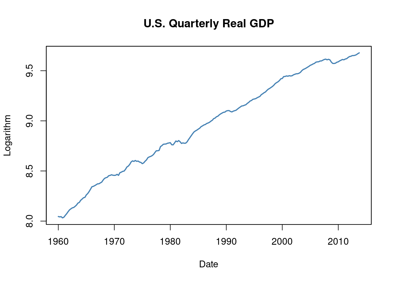
The dataset us_macro_quarterly.xlsx contains quarterly data on U.S. real GDP (inflation-adjusted) from 1947 to 2004.
The first column contains text, while the remaining columns are numeric. We can specify the column types by using col_types = c("text", rep("numeric", 9)) when reading the data.
# load US macroeconomic data
USMacroSWQ <- read_xlsx("us_macro_quarterly.xlsx",
                         sheet = 1,
                         col_types = c("text", rep("numeric", 9)))

# format date column
USMacroSWQ$...1 <- as.yearqtr(USMacroSWQ$...1, format = "%Y:0%q")

# adjust column names
colnames(USMacroSWQ) <- c("Date", "GDPC96", "JAPAN_IP", "PCECTPI",
                          "GS10", "GS1", "TB3MS", "UNRATE", "EXUSUK", "CPIAUCSL")
6.2 Time Series Data and Serial Correlation
Working with time-series objects that track the frequency of the data and are extensible is useful for an effective time series analysis. We will use objects of the class xts for this purpose, which have a time-based ordered index. See ?xts.
The data in USMacroSWQ are in quarterly frequency, so we convert the first column to yearqtr format before generating the xts object GDP.
As with any data analysis, a good starting point is to visualize the data. For this purpose, we will use the quantmod package, which offers convenient functions for plotting and computing with time series data.
6.3 Lags, Differences, Logarithms and Growth Rates
For observations of a variable Y recorded over time, Y_t represents the value observed at time t. The interval between two consecutive observations, Y_{t-1} and Y_t, defines a unit of time (e.g. hours, days, weeks, months, quarters or years).
Previous values of a time series are called lags. The first lag of Y_t is Y_{t-1}. The j^{th} lag of Y_t is Y_{t-j}. In R, lags of univariate or multivariate time series objects are computed by lag() (see ?lag).
It is sometimes convenient to work with a differenced series. The first difference of a series is \Delta Y_t = Y_t - Y_{t-1}. For a time series Y, we compute the series of first differences as diff(Y) in R.
Since it is common to report growth rates in macroeconomic series, it is convenient to work with the first difference in logarithms of a series, denoted by \Delta \log(Y_t) = \log(Y_t) - \log(Y_{t-1}). We can obtain this in R by using log(Y/lag(Y)).
We may additionally approximate the percentage change between Y_t and Y_{t-1} as 100\Delta\log(Y_t).
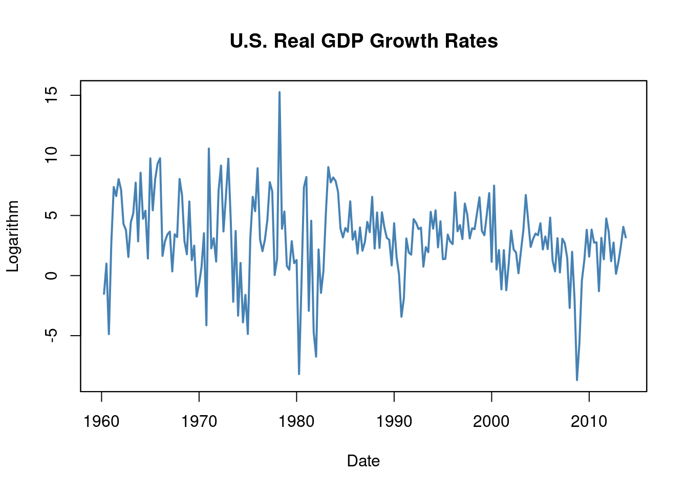
We can now present the quarterly U.S. GDP time series, its logarithm, the annualized growth rate and the first lag of the annualized growth rate series for the period 2012:Q1 - 2013:Q1. The following function quants can be used to compute these quantities for a quarterly time series.
Since 100\Delta\log(Y_t) is an approximation of the quarterly percentage changes, we compute the annual growth rate using the approximation
\text{AnnualGrowth}Y_t = 400 \cdot \Delta \log(Y_t)
We may now call quants() on observations for the period 2011:Q3 - 2013:Q1.
# obtain a data.frame with level, logarithm, annual growth rate and its 1st lag of GDP
quants(GDP["2011-07::2013-01"])
Level Logarithm AnnualGrowthRate X1stLagAnnualGrowthRate
2011 Q3 15062.14 9.619940 NA NA
2011 Q4 15242.14 9.631819 4.7518062 NA
2012 Q1 15381.56 9.640925 3.6422231 4.7518062
2012 Q2 15427.67 9.643918 1.1972004 3.6422231
2012 Q3 15533.99 9.650785 2.7470216 1.1972004
2012 Q4 15539.63 9.651149 0.1452808 2.7470216
2013 Q1 15583.95 9.653997 1.1392015 0.14528086.4 Autocorrelation
Observations of a time series are typically correlated. This is called autocorrelation or serial correlation.
We can compute the first four sample autocorrelations of the series GDPGrowth using acf().
Autocorrelations of series 'na.omit(GDPGrowth)', by lag

 0.00  0.25  0.50  0.75  1.00
1.000 0.352 0.273 0.114 0.106
These values suggest a mild positive autocorrelation in GDP growth: when GDP grows faster than average in one period, it tends to continue growing faster than average in subsequent periods.
6.5 Additional Examples of Economic Time Series
The book by Stock and Watson (2020, Global Edition) presents four plots in figure 15.2: the U.S. unemployment rate, the U.S. Dollar / British Pound exchange rate, the logarithm of the Japanese industrial production index and daily changes in the Wilshire 5000 stock price index, a financial time series.
To reproduce these plots, we additionally use the data set NYSESW included in the AER package. We now plot the three macroeconomic series and add percentage changes in the daily values of the New York Stock Exchange Composite index as a fourth plot.
# define series as xts objects
USUnemp <- xts(USMacroSWQ$UNRATE, USMacroSWQ$Date)["1960::2013"]

DollarPoundFX <- xts(USMacroSWQ$EXUSUK, USMacroSWQ$Date)["1960::2013"]

JPIndProd <- xts(log(USMacroSWQ$JAPAN_IP), USMacroSWQ$Date)["1960::2013"]

# attach NYSESW data
data("NYSESW")
NYSESW <- xts(Delt(NYSESW))
# divide plotting area into 2x2 matrix
par(mfrow = c(2, 2))
# plot the series
plot(as.zoo(USUnemp),
col = "steelblue",
lwd = 2,
ylab = "Percent",
xlab = "Date",
main = "US Unemployment Rate",
cex.main = 0.8)
plot(as.zoo(DollarPoundFX),
col = "steelblue",
lwd = 2,
ylab = "Dollar per pound",
xlab = "Date",
main = "U.S. Dollar / B. Pound Exchange Rate",
cex.main = 0.8)
plot(as.zoo(JPIndProd),
col = "steelblue",
lwd = 2,
ylab = "Logarithm",
xlab = "Date",
main = "Japanese Industrial Production",
cex.main = 0.8)
plot(as.zoo(NYSESW),
col = "steelblue",
lwd = 2,
ylab = "Percent per Day",
xlab = "Date",
main = "New York Stock Exchange Composite Index",
cex.main = 0.8)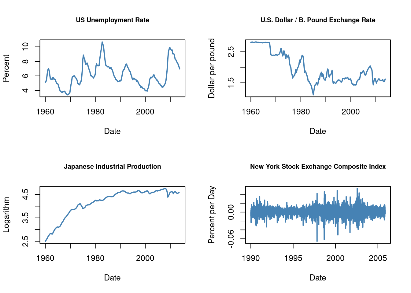
We observe different characteristics in the series:
The unemployment rate rises during recessions and falls during periods of economic recovery and growth.
The Dollar/Pound exchange rate followed a deterministic pattern until the Bretton Woods system ended.
Japan’s industrial production shows an upward trend with diminishing growth.
Daily changes in the New York Stock Exchange composite index appear to fluctuate randomly around zero. The sample autocorrelations support this observation.
Autocorrelations of series 'na.omit(NYSESW)', by lag

     0      1      2      3      4      5      6      7      8      9     10
 1.000  0.040 -0.016 -0.023  0.000 -0.036 -0.027 -0.059  0.013  0.017  0.004
The first 10 sample autocorrelation coefficients are nearly zero. The default plot produced by acf() offers additional confirmation.
# plot sample autocorrelation for the NYSESW series
acf(na.omit(NYSESW), main = "Sample Autocorrelation for NYSESW Data")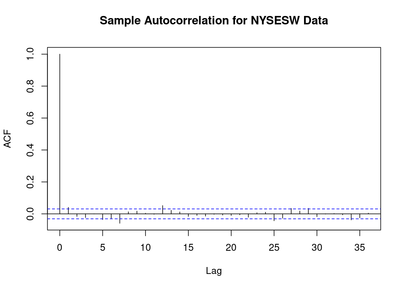
The blue dashed bands represent values beyond which the autocorrelations are significantly different from zero at 5\% level. For most lags, the sample autocorrelation remains within the bands, with only a few instances slightly exceeding the limits.
Additionally, the NYSESW series show volatility clustering, characterized by periods of high and low variance. This pattern is typically observed in many financial time series.
6.6 Autoregressions
6.6.1 The First-Order Autoregressive Model
The simplest autoregressive model uses only the most recent outcome of the time series observed to predict future values. For a time series Y_t, this model is known as a first-order autoregressive model, commonly abbreviated as AR(1).
Y_t = \beta_0 + \beta_1 Y_{t-1} + u_t is the AR(1) population model of a time series Y_t.
The first-order autoregression model of GDP growth can be estimated by computing OLS estimates in the regression of GDPGR_t on GDPGR_{t-1}
\widehat{GDPGR}_t = \hat{\beta}_0 + \hat{\beta}_1 GDPGR_{t-1}
To estimate this regression model, we use data from 1962 to 2012 and we use ar.ols() from the package stats.
# subset data
GDPGRSub <- GDPGrowth["1962::2012"]

# estimate the model
ar.ols(GDPGRSub,
       order.max = 1,
       demean = F,
       intercept = T)
Call:
ar.ols(x = GDPGRSub, order.max = 1, demean = F, intercept = T)

Coefficients:
     1
0.3384

Intercept: 1.995 (0.2993)

Order selected 1  sigma^2 estimated as  9.886
We see that the computations done by ar.ols() are the same as done by lm().
# length of data set
N <-length(GDPGRSub)

GDPGR_level <- as.numeric(GDPGRSub[-1])
GDPGR_lags <- as.numeric(GDPGRSub[-N])

# estimate the model
armod <- lm(GDPGR_level ~ GDPGR_lags)
armod
Call:
lm(formula = GDPGR_level ~ GDPGR_lags)

Coefficients:
(Intercept)   GDPGR_lags
     1.9950       0.3384
We obtain a robust summary on the estimated regression coefficients as usual with coeftest().
# robust summary
coeftest(armod, vcov. = vcovHC, type = "HC1")
t test of coefficients:

            Estimate Std. Error t value  Pr(>|t|)
(Intercept) 1.994986   0.351274  5.6793 4.691e-08 ***
GDPGR_lags  0.338436   0.076188  4.4421 1.470e-05 ***
---
Signif. codes:  0 '***' 0.001 '**' 0.01 '*' 0.05 '.' 0.1 ' ' 1
The estimated regression model is
\widehat{GDPGR_t} = \underset{(0.351)}{1.995} + \underset{(0.076)}{0.338} \, GDPGR_{t-1}.
We omit the first observation for GDPGR_{1962 \, Q1} from the vector of the dependent variable since GDPGR_{1962 \, Q1-1} = GDPGR_{1961 \, Q4} is not included in the sample. Similarly, the last observation, GDPGR_{2012 \, Q4} is excluded from the predictor vector since the data does not include GDPGR_{2012 \, Q4 + 1} = GDPGR_{2013 \, Q1}.
Put differently, when estimating the model, one observation is lost because of the time series structure of the data.
6.6.2 Forecasts and Forecast Errors
When Y_t follows an AR(1) model with an intercept and we have an OLS estimate of the model on the basis of observations for T periods, then we may use the AR(1) model to obtain \widehat Y_{T+1|T}, a forecast for Y_{T+1} using data up to period T, where
\widehat{Y}_{T+1|T} = \widehat{\beta}_0 + \widehat{\beta}_1 Y_T.
The forecast error is then
\text{Forecast error} = Y_{T+1} - \widehat{Y}_{T+1|T}
6.6.3 Forecasts and Forecasted Values
Forecasted values of Y_t are different from what we call OLS predicted values of Y_t. Additionally, the forecast error differs from an OLS residual. Forecasts and forecast errors are derived using out-of-sample data, whereas predicted values and residuals are calculated using in-sample data that has been observed.
The root mean squared forecast error (RMSFE) quantifies the typical magnitude of the forecast error and is defined as
\text{RMSFE} = \sqrt{E\left[ \left(Y_{T+1} - \widehat{Y}_{T+1|T}\right)^2 \right]}
The RMSFE consists of future errors u_t and the error derived from estimating the coefficients. When the sample size is large, the future errors often dominate, making RMSFE approximately equal to \sqrt{\text{Var}(u_t)}, which can be estimated by the standard error of the regression.
6.6.4 Application to GDP Growth
Using the estimated AR(1) model of GDP growth, we can perform the forecast for the GDP growth for the first quarter of 2013. Since we estimated the model using data from 1962:Q1 to 2012:Q4, 2013:Q1 is an out-of-sample period.
Substituting GDPGR_{2012 \, Q4} \approx 0.15 into the equation, we obtain:
\widehat{GDPGR}_{2013:Q1} = 1.995 + 0.348 \cdot 0.15 = 2.047
The forecast() function from the forecast package provides useful features for making time series predictions.
# assign GDP growth rate in 2012:Q4
new <- data.frame("GDPGR_lags" = GDPGR_level[N-1])

# forecast GDP growth rate in 2013:Q1
forecast(armod, newdata = new)
Point Forecast Lo 80 Hi 80 Lo 95 Hi 95
1 2.044155 -2.036225 6.124534 -4.213414 8.301723We observe the same point forecast of approximately 2.0, together with the 80\% and 95\% forecast intervals.
We conclude that the AR(1) model predicts the GDP growth to be 2\% in 2013:Q1.
But how reliable is this forecast? The forecast error is substantial: GDPGR_{2013 \,Q1} \approx 1.1\%, while our prediction is 2\%. Additionally, using summary(armod) reveals that the model accounts for only a small portion of the GDP growth rate variation, with the SER around 3.16. Ignoring the forecast uncertainty from estimating coefficients \beta_0 and \beta_1, the RMSFE should be at least 3.16\%, which is the estimated standard deviation of the errors. Thus, we conclude that this forecast is quite inaccurate.
# compute the forecast error
forecast(armod, newdata = new)$mean - GDPGrowth["2013"][1]
x
2013 Q1 0.9049532# R^2
summary(armod)$r.squared[1] 0.1149576# SER
summary(armod)$sigma[1] 3.159796.6.5 Autoregressive Models of Order p
The AR(1) model only considers information from the most recent period to forecast GDP growth. In contrast, an AR(p) model includes information from the past p lags of the series.
An AR(p) model assumes that a time series Y_t can be modeled by a linear function of the first p of its lagged values.
Y_t = \beta_0 + \beta_1 Y_{t-1} + \beta_2 Y_{t-2} + \cdots + \beta_p Y_{t-p} + u_t
is an autoregressive model of order p where E(u_t \mid Y_{t-1}, Y_{t-2}, \ldots, Y_{t-p}) = 0.
Let’s estimate an AR(2) model of the GDP growth series from 1962:Q1 to 2012:Q4.
# estimate the AR(2) model
GDPGR_AR2 <- dynlm(ts(GDPGR_level) ~ L(ts(GDPGR_level)) + L(ts(GDPGR_level), 2))

coeftest(GDPGR_AR2, vcov. = sandwich)
t test of coefficients:

                      Estimate Std. Error t value  Pr(>|t|)
(Intercept)           1.631747   0.402023  4.0588 7.096e-05 ***
L(ts(GDPGR_level))    0.277787   0.079250  3.5052 0.0005643 ***
L(ts(GDPGR_level), 2) 0.179269   0.079951  2.2422 0.0260560 *
---
Signif. codes:  0 '***' 0.001 '**' 0.01 '*' 0.05 '.' 0.1 ' ' 1
We obtain
\widehat{GDPGR_t} = \underset{(0.40)}{1.63} + \underset{(0.08)}{0.28} \, GDPGR_{t-1} + \underset{(0.08)}{0.18} \, GDPGR_{t-2}
We see that the coefficient on the second lag is significantly different from zero at the 5\% level. Compared to the AR(1) model, the fit shows a slight improvement: \bar R^2 increases from 0.11 in the AR(1) model to about 0.14 in the AR(2), and the SER decreases to 3.13.
We can use the AR(2) model to forecast GDP growth for 2013 in the same way as we did with the AR(1) model.
# AR(2) forecast of GDP growth in 2013:Q1
forecast <- c("2013:Q1" = coef(GDPGR_AR2) %*% c(1, GDPGR_level[N-1],
                                                GDPGR_level[N-2]))
forecast
2013:Q1
2.16456 The forecast error is approximately -1\%.
# compute AR(2) forecast error
GDPGrowth["2013"][1] - forecast
x
2013 Q1 -1.0253586.7 Additional Predictors and The ADL Model
An autoregressive distributed lag (ADL) model is called autoregressive because it includes lagged values of the dependent variable as regressors (similar to an autoregression), but it’s also termed a distributed lag model because the regression incorporates multiple lags (a “distributed lag”) of an additional predictor.
The autoregressive distributed lag model with p lags of Y_t and q lags of X_t, denoted ADL(p, q), is
\begin{align*} Y_t &= \beta_0 + \beta_1 Y_{t-1} + \beta_2 Y_{t-2} + \cdots + \beta_p Y_{t-p} \\ &\quad + \delta_1 X_{t-1} + \delta_2 X_{t-2} + \cdots + \delta_q X_{t-q} + u_t \end{align*}
where \beta_0, \beta_1, \ldots, \beta_p, \delta_1, \ldots, \delta_q, are unknown coefficients and u_t is the error term with E(u_t \mid Y_{t-1}, Y_{t-2}, \ldots, X_{t-1}, X_{t-2}, \ldots) = 0.
6.7.1 Forecasting GDP Growth Using the Term Spread
Interest rates on long-term and short-term treasury bonds are closely tied to macroeconomic conditions. Although both types of bonds share similar long-term trends, their short-term behaviors differ significantly. The disparity in interest rates between two bonds with different maturities is known as the term spread.
Figure 15.3 of the book by Stock and Watson (2020, Global Edition) displays interest rates of 10-year U.S. Treasury bonds and 3-month U.S. Treasury bills from 1960 to 2012. The following code chunks reproduce this figure.
# reproduce Figure 15.3 (a) of the book
plot(merge(as.zoo(TB3MS), as.zoo(TB10YS)),
     plot.type = "single",
     col = c("darkred", "steelblue"),
     lwd = 2,
     xlab = "Date",
     ylab = "Percent per annum",
     main = "10-year and 3-month Interest Rates")

# define function that transform years to class 'yearqtr'
YToYQTR <- function(years) {
  return(
      sort(as.yearqtr(sapply(years, paste, c("Q1", "Q2", "Q3", "Q4"))))
  )
}

# recessions
recessions <- YToYQTR(c(1961:1962, 1970, 1974:1975, 1980:1982, 1990:1991, 2001,
                        2007:2008))

# add color shading for recessions
xblocks(time(as.zoo(TB3MS)),
        c(time(TB3MS) %in% recessions),
        col = alpha("steelblue", alpha = 0.3))

# add a legend
legend("topright",
       legend = c("TB3MS", "TB10YS"),
       col = c("darkred", "steelblue"),
       lwd = c(2, 2))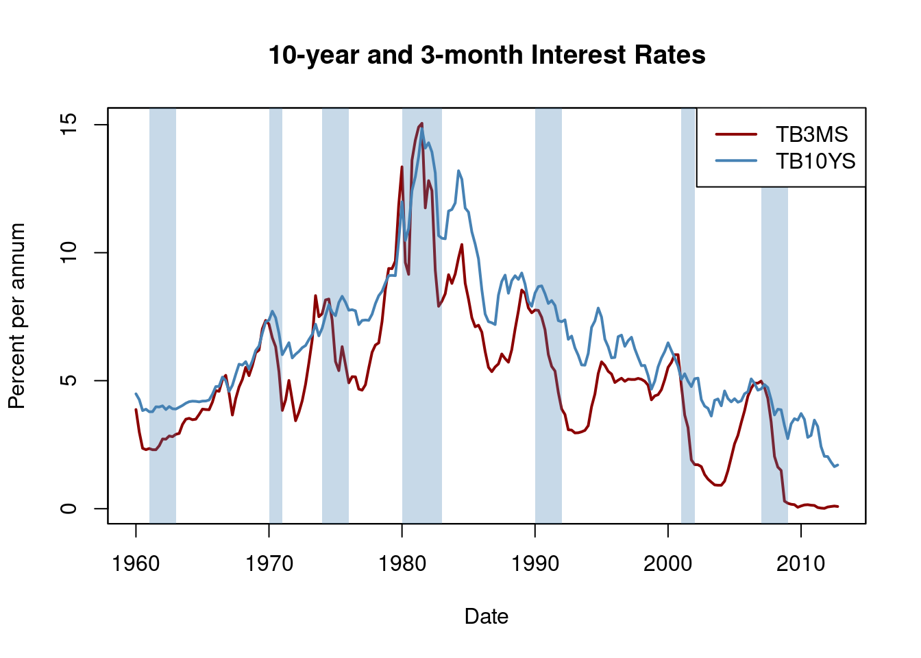
# reproduce Figure 15.3 (b) of the book
plot(as.zoo(TSpread),
     col = "steelblue",
     lwd = 2,
     xlab = "Date",
     ylab = "Percent per annum",
     main = "Term Spread")

# add color shading for recessions
xblocks(time(as.zoo(TB3MS)),
        c(time(TB3MS) %in% recessions),
        col = alpha("steelblue", alpha = 0.3))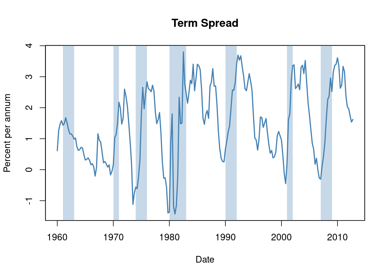
Before recessions, the gap between interest rates on long-term bonds and short-term bills narrows, causing the term spread to decline significantly, sometimes even turning negative during economic stress. This information can be used to improve future GDP growth forecasts.
We can verify this by estimating an ADL(2, 1) model and an ADL(2, 2) model of the GDP growth rate, using lags of GDP growth and lags of the term spread as regressors. Then we use both models to forecast GDP growth for 2013.
# estimate the ADL(2,1) model of GDP growth
GDPGR_ADL21 <- dynlm(GDPGrowth_ts ~ L(GDPGrowth_ts) + L(GDPGrowth_ts, 2) +
                       L(TSpread_ts), start = c(1962, 1), end = c(2012, 4))

coeftest(GDPGR_ADL21, vcov. = sandwich)
t test of coefficients:

                   Estimate Std. Error t value Pr(>|t|)
(Intercept)        0.954990   0.486976  1.9611 0.051260 .
L(GDPGrowth_ts)    0.267729   0.082562  3.2428 0.001387 **
L(GDPGrowth_ts, 2) 0.192370   0.077683  2.4763 0.014104 *
L(TSpread_ts)      0.444047   0.182637  2.4313 0.015925 *
---
Signif. codes:  0 '***' 0.001 '**' 0.01 '*' 0.05 '.' 0.1 ' ' 1
We obtain for ADL (2,1) the following equation
\widehat {GDPGR_t} = \underset{(0.49)}{0.96} + \underset{(0.08)}{0.26} \, GDPGR_{t-1} + \underset{(0.08)}{0.19} \, GDPGR_{t-2} + \underset{(0.18)}{0.44} \, TSpread_{t-1}
with all coefficients significant at the 5\% level.
Let’s now predict the GDP growth for 2013:Q1 and compute the forecast error.
# 2012:Q3 / 2012:Q4 data on GDP growth and term spread
subset <- window(ADLdata, c(2012, 3), c(2012, 4))

# ADL(2,1) GDP growth forecast for 2013:Q1
ADL21_forecast <- coef(GDPGR_ADL21) %*% c(1, subset[2, 1], subset[1, 1],
                                          subset[2, 2])
ADL21_forecast
[,1]
[1,] 2.241689 Qtr1
2013 -1.102487The ADL(2,1) model predicts the GDP growth in 2013:Q1 to be 2.24\%, which leads to a forecast error of -1.10\%.
We now estimate the ADL(2, 2) model to determine if incorporating additional information from past term spreads enhances the forecast.
# estimate the ADL(2,2) model of GDP growth
GDPGR_ADL22 <- dynlm(GDPGrowth_ts ~ L(GDPGrowth_ts) + L(GDPGrowth_ts, 2)
                     + L(TSpread_ts) + L(TSpread_ts, 2),
                     start = c(1962, 1), end = c(2012, 4))

coeftest(GDPGR_ADL22, vcov. = sandwich)
t test of coefficients:

                    Estimate Std. Error t value Pr(>|t|)
(Intercept)         0.967967   0.472470  2.0487 0.041800 *
L(GDPGrowth_ts)     0.243175   0.077836  3.1242 0.002049 **
L(GDPGrowth_ts, 2)  0.177070   0.077027  2.2988 0.022555 *
L(TSpread_ts)      -0.139554   0.422162 -0.3306 0.741317
L(TSpread_ts, 2)    0.656347   0.429802  1.5271 0.128326
---
Signif. codes:  0 '***' 0.001 '**' 0.01 '*' 0.05 '.' 0.1 ' ' 1
The estimated AR(2,2) model equation is
\begin{align*} \widehat{GDPGR}_t &= \underset{(0.47)}{0.98} + \underset{(0.08)}{0.24} \, GDPGR_{t-1} + \underset{(0.08)}{0.18} \, GDPGR_{t-2} \\ &\quad - \underset{(0.42)}{0.14} \, TSpread_{t-1} + \underset{(0.43)}{0.66} \, TSpread_{t-2} \end{align*}
While the coefficients on the lagged growth rates are still significant, the coefficients on both lags of the term spread are not significant at the 10\% level.
# ADL(2,2) GDP growth forecast for 2013:Q1
ADL22_forecast <- coef(GDPGR_ADL22) %*% c(1, subset[2, 1], subset[1, 1],
                                          subset[2, 2], subset[1, 2])
ADL22_forecast
[,1]
[1,] 2.274407 Qtr1
2013 -1.135206The ADL(2,2) model forecasts a GDP growth of 2.27\% for 2013:Q1, which implies a forecast error of -1.14\%.
Are ADL(2,1) and ADL(2,2) models better than the simple AR(2) model? Yes, while SER and \bar R^2 improve only slightly, an F-test on the term spread coefficients in the ADL(2,2) model provides evidence that the model does better in explaining GDP growth than the AR(2) model, as the hypothesis that both coefficients are zero can be rejected at the 5\% level.
# compare adj. R2
c("Adj.R2 AR(2)" = summary(GDPGR_AR2)$adj.r.squared,
  "Adj.R2 ADL(2,1)" = summary(GDPGR_ADL21)$adj.r.squared,
  "Adj.R2 ADL(2,2)" = summary(GDPGR_ADL22)$adj.r.squared)
Adj.R2 AR(2) Adj.R2 ADL(2,1) Adj.R2 ADL(2,2)
0.1338873 0.1620156 0.1691531 # compare SER
c("SER AR(2)" = summary(GDPGR_AR2)$sigma,
"SER ADL(2,1)" = summary(GDPGR_ADL21)$sigma,
"SER ADL(2,2)" = summary(GDPGR_ADL22)$sigma) SER AR(2) SER ADL(2,1) SER ADL(2,2)
3.132122 3.070760 3.057655 # F-test on coefficients of term spread
linearHypothesis(GDPGR_ADL22,
c("L(TSpread_ts)=0", "L(TSpread_ts, 2)=0"),
vcov. = sandwich)Linear hypothesis test
Hypothesis:
L(TSpread_ts) = 0
L(TSpread_ts, 2) = 0
Model 1: restricted model
Model 2: GDPGrowth_ts ~ L(GDPGrowth_ts) + L(GDPGrowth_ts, 2) + L(TSpread_ts) +
L(TSpread_ts, 2)
Note: Coefficient covariance matrix supplied.
Res.Df Df F Pr(>F)
1 201
2 199 2 4.4344 0.01306 *
---
Signif. codes: 0 '***' 0.001 '**' 0.01 '*' 0.05 '.' 0.1 ' ' 16.7.2 Stationarity
Time series forecasts rely on past data to predict future values, assuming that the correlations and distributions of the data will remain consistent over time. This assumption is formalized by the concept of stationarity.
A time series Y_t is stationary if its probability distribution does not change over time - that is, if the joint distribution of (Y_{s+1}, Y_{s+2}, \ldots, Y_{s+T}) does not depend on s, regardless of the value of T; otherwise, Y_t is said to be nonstationary.
Similarly, a pair of time series, X_t and Y_t, are said to be jointly stationary if the joint distribution of (X_{s+1}, Y_{s+1}, X_{s+2}, Y_{s+2}, \ldots, X_{s+T}, Y_{s+T}) does not depend on s, regardless of the value of T.
6.7.3 Time Series Regression with Multiple Predictors
The general time series regression model extends the ADL model to include multiple regressors and their lags. It incorporates p lags of the dependent variable and q_l lags of l additional predictors where l = 1, \ldots, k:
\begin{align*} Y_t &= \beta_0 + \beta_1 Y_{t-1} + \beta_2 Y_{t-2} + \cdots + \beta_p Y_{t-p} \\ &\quad + \delta_{11} X_{1,t-1} + \delta_{12} X_{1,t-2} + \cdots + \delta_{1q} X_{1,t-q} \\ &\quad + \cdots \\ &\quad + \delta_{k1} X_{k,t-1} + \delta_{k2} X_{k,t-2} + \cdots + \delta_{kq} X_{k,t-q} \\ &\quad + u_t. \end{align*}
The following assumptions are made for estimation:
- The error term u_t has conditional mean zero given all regressors and their lags:
E(u_t \mid Y_{t-1}, Y_{t-2}, \ldots, X_{1,t-1}, X_{1,t-2}, \ldots, X_{k,t-1}, X_{k,t-2}, \ldots)
This assumption extends the conditional mean zero assumption used for AR and ADL models and ensures that the general time series regression model described above provides the optimal forecast of Y_t given its lags, the additional regressors X_{1,t}, \ldots, X_{k,t}, and their lags.
-
The i.i.d. assumption for cross-sectional data is not entirely applicable to time series data. Instead, we replace it with the following assumption, which has two components:
The (Y_t, X_{1,t}, \ldots, X_{k,t}) have a stationary distribution (the “identically distributed” part of the i.i.d. assumption for cross-sectional data). If this condition does not hold, forecasts may be biased and inference can be significantly misleading.
The (Y_t, X_{1,t}, \ldots, X_{k,t}) and (Y_{t-j}, X_{1,t-j}, \ldots, X_{k,t-j}) become independent as j becomes large (the “independently” distributed part of the i.i.d. assumption for cross-sectional data). This assumption is also referred to as weak dependence and ensures that the WLLN and the CLT hold in large samples.
Large outliers are unlikely: E(X_{1,t}^4), E(X_{2,t}^4), \ldots, E(X_{k,t}^4) and E(Y_t^4) have nonzero, finite fourth moments.
No perfect multicollinearity.
Given the nonstationary nature observed in many economic time series, assumption two plays a crucial role in applied macroeconomics and finance, leading to the development of statistical tests designed to determine stationarity or nonstationarity that will be explained later.
6.7.4 Statistical Inference and the Granger Causality Test
If X serves as a valuable predictor for Y, then in a regression where Y_t is regressed on its own lags and lags of X_t, some coefficients on the lags of X_t are expected to be non-zero. This concept is known as Granger causality and presents an interesting hypothesis for testing.
The Granger causality test is an F-test of the null hypothesis that all lags of a variable X included in a time series regression model do not have predictive power for Y_t. It does not test whether X actually causes Y, but whether the included lags are informative in terms of predicting Y.
This is the test we have previously performed on the ADL(2,2) model of GDP growth and we concluded that at least one of the first two lags of term spread has predictive power for GDP growth.
6.8 Forecast Uncertainty and Forecast Intervals
It is typically good practice to include a measure of uncertainty when presenting results affected by it. Uncertainty becomes especially important in the context of time series forecasting.
For instance, consider a basic ADL(1,1) model
Y_t = \beta_0 + \beta_1 Y_{t-1} + \delta_1 X_{t-1} + u_t,
where u_t is a homoskedastic error term. The forecast error is then
Y_{T+1} - \widehat{Y}_{T+1 \mid T} = u_{T+1} - [ (\widehat{\beta}_0 - \beta_0) + (\widehat{\beta}_1 - \beta_1) Y_T + (\widehat{\delta_1} - \delta_1) X_T ]
The mean squared forecast error (MSFE) and the RMSFE are
\begin{align*} MSFE &= E \left[ (Y_{T+1} - \widehat{Y}_{T+1 \mid T})^2 \right] \\ &= \sigma^2_u + Var \left[ (\widehat{\beta}_0 - \beta_0) + (\widehat{\beta}_1 - \beta_1) Y_T + (\widehat{\delta}_1 - \delta_1) X_T \right], \\ RMSE &= \sqrt{\sigma^2_u + \text{Var} \left[ (\widehat{\beta}_0 - \beta_0) + (\widehat{\beta}_1 - \beta_1) Y_T + (\widehat{\delta}_1 - \delta_1) X_T \right]}. \end{align*}
A 95\% forecast interval is an interval that, in 95\% of repeated applications, includes the true value of Y_{T+1}.
There is a fundamental distinction between computing a confidence interval and a forecast interval. When deriving a confidence interval for a point estimate, we use large sample approximations justified by the Central Limit Theorem (CLT), and these are valid across a broad range of error term distributions.
On the other hand, to compute a forecast interval for Y_{T+1}, an additional assumption about the distribution of u_{T+1}, the error term in period T+1, is necessary.
Assuming that u_{T+1} follows a normal distribution, it is possible to create a 95\% forecast interval for Y_{T+1} using SE(Y_{T+1} - \hat{Y}_{T+1|T}), which represents an estimate of the Root Mean Squared Forecast Error (RMSFE).
\hat{Y}_{T+1|T} \pm 1.96 \cdot SE(Y_{T+1} - \hat{Y}_{T+1|T})
Nevertheless, the computation gets more complicated when the error term is heteroskedastic or if we are interested in computing a forecast interval for T+s when s > 1.
In some cases it is useful to report multiple forecast intervals for subsequent periods. To ilustrate an example, we will use simulated time series data and estimate an AR(2) model which is then used for forecasting the subsequent 25 future outcomes of the series.
# set seed
set.seed(1234)

# simulate the time series
Y <- arima.sim(list(order = c(2, 0, 0), ar = c(0.2, 0.2)),  n = 200)

# estimate an AR(2) model using 'arima()', see ?arima
model <- arima(Y, order = c(2, 0, 0))

# compute points forecasts and prediction intervals for the next 25 periods
fc <- forecast(model, h = 25, level = seq(5, 99, 10))

# plot a fan chart
plot(fc,
     main = "Forecast Fan Chart for AR(2) Model of Simulated Data",
     showgap = F,
     fcol = "red",
     flty = 2)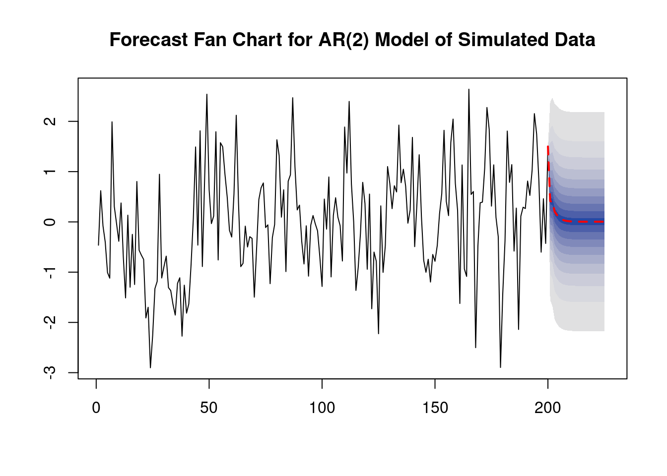
arima.sim() simulates autoregressive integrated moving average (ARIMA) models. These are the class of models AR models belong to.
We use list(order = c(2, 0, 0), ar = c(0.2, 0.2)) so the data generating process (DGP) is
Y_t = 0.2 Y_{t-1} + 0.2 Y_{t-2} + u_t.
We choose level = seq(5, 99, 10) in the call of forecast() so that forecast intervals with levels 5\%, 15\%,\ldots, 95\% are computed for each point forecast of the series.
The dashed red line displays the series’ point forecasts for the next 25 periods using an AR(2) model, while the shaded areas represent prediction intervals.
The shading intensity corresponds to the interval’s level, with the darkest blue band representing the 5\% forecast intervals, gradually fading to grey with higher interval levels.
6.9 Lag Length Selection using Information Criteria
The determination of lag lengths in AR and ADL models may be influenced by economic theory, yet statistical techniques are useful in selecting the appropriate number of lags as regressors.
Including too many lags typically inflates the standard errors of coefficient estimates, leading to increased forecast errors, whereas omitting essential lags can introduce estimation biases into the model.
The order of an AR model can be determined using two approaches:
- The F-test approach
Estimate an AR(p) model and test the significance of its largest lag(s). If statistical tests suggest that certain lag(s) are not significant, we may consider removing them from the model. However, this method often leads to overfitting, as significance tests can sometimes incorrectly reject a true null hypothesis.
- Relying on an information criterion
To avoid the problem of overly complex models, one can select the lag order that minimizes one of the following two information criteria:
- The Bayes Information Criterion (BIC):
BIC(p) = \log\left(\frac{SSR(p)}{T}\right) + (p + 1) \frac{\log(T)}{T}
- The Akaike Information Criterion (AIC):
AIC(p) = \log\left(\frac{SSR(p)}{T}\right) + (p + 1) \frac{2}{T}
Both criteria are estimators of the optimal lag length p. The lag order \hat p that minimizes the respective criterion is called the BIC estimate or the AIC estimate of the optimal model order.
The basic idea of both criteria is that the SSR decreases as additional lags are added to the model, such that the first term decreases whereas the second increases as the lag order grows.
BIC decreases because of its logarithmic penalty term, while AIC’s penalty term is less severe. BIC is consistent in estimating the true lag order, whereas AIC’s consistency is less assured due to its different penalty factor.
Despite this, both criteria are commonly employed, with AIC sometimes favored when BIC suggests a model with too few lags.
The dynlm() function does not compute information criteria by default. Hence, we will create a custom function to calculate and display the Bayesian Information Criterion (BIC), alongside the selected lag order p and the adjusted \bar R^2, for objects of class dynlm.
The following code computes the Bayesian Information Criterion (BIC) for autoregressive (AR) models of GDP growth with orders p = 1, \ldots, 6.
sapply() function is used to apply the BIC calculation to each model and display the results, including the BIC values and the adjusted \bar R^2 for each order. This allows for a comparison of model fit across different lag lengths.
     p    BIC Adj.R2
0.0000 2.4394 0.0000
# loop BIC over models of different orders
order <- 1:6
BICs <- sapply(order, function(x)
"AR" = BIC(dynlm(ts(GDPGR_level) ~ L(ts(GDPGR_level), 1:x))))
BICs [,1] [,2] [,3] [,4] [,5] [,6]
p 1.0000 2.0000 3.0000 4.0000 5.0000 6.0000
BIC 2.3486 2.3475 2.3774 2.4034 2.4188 2.4429
Adj.R2 0.1099 0.1339 0.1303 0.1303 0.1385 0.1325Increasing the lag order tends to increase R^2 because adding more lags generally reduces the sum of squared residuals SSR. However, \bar R^2 adjusts for the number of parameters in the model, mitigating the inflation of R^2 due to additional variables.
Despite \bar R^2 considerations, according to the BIC criterion, opting for the AR(2) model over the AR(5) model is recommended. The BIC helps in assessing whether the reduction in SSR justifies the inclusion of an additional regressor.
If we had to compare a bigger set of models, we may use the function which.min() to select the model with the lowest BIC.
# select the AR model with the smallest BIC
BICs[, which.min(BICs[2, ])]
p BIC Adj.R2
2.0000 2.3475 0.1339 The BIC may also be used to select lag lengths in time series regression models with multiple predictors. In a model with K coefficients, including the intercept, we have
\text{BIC}(K) = \log \left( \frac{SSR(K)}{T} \right) + K \frac{\log(T)}{T}.
Choosing the optimal model according to the BIC can be computationally demanding, since there may be many different combinations of lag lengths when there are multiple predictors.
As an example, we estimate ADL(p,q) models of GDP growth, incorporating the term spread between short-term and long-term bonds as an additional variable.
We impose the constraint p= q_1 = \ldots = q_k so that only a maximum of p_{\text{max}} models (p = 1, \ldots, p_{\text{max}}) need to be estimated. In the example below, we set p_{\text{max}}=12.
# loop 'BIC()' over multiple ADL models
order <- 1:12

BICs <- sapply(order, function(x)
         BIC(dynlm(GDPGrowth_ts ~ L(GDPGrowth_ts, 1:x) + L(TSpread_ts, 1:x),
                   start = c(1962, 1), end = c(2012, 4))))

BICs
[,1] [,2] [,3] [,4] [,5] [,6] [,7] [,8] [,9]
p 2.0000 4.0000 6.0000 8.0000 10.0000 12.0000 14.0000 16.0000 18.0000
BIC 2.3411 2.3408 2.3813 2.4181 2.4568 2.5048 2.5539 2.6029 2.6182
Adj.R2 0.1332 0.1692 0.1704 0.1747 0.1773 0.1721 0.1659 0.1586 0.1852
[,10] [,11] [,12]
p 20.0000 22.0000 24.0000
BIC 2.6646 2.7205 2.7664
Adj.R2 0.1864 0.1795 0.1810According to the definition of BIC(), for ADL models where p=q, p represents the count of estimated coefficients excluding the intercept. Consequently, the lag order is derived by dividing p by 2.
# select the ADL model with the smallest BIC
BICs[, which.min(BICs[2, ])]
p BIC Adj.R2
4.0000 2.3408 0.1692 The BIC favors the previously estimated ADL(2, 2) model.