2 Empirical Applications in Panel Data Analysis
Welcome to the first empirical application in R! Here you will have the opportunity to bridge theory with practice by applying the concepts to real-world datasets available in R. This will help you better understanding the theory and hopefully motivate you to keep conducting your own applications in R.
Our journey begins always with a brief overview of each dataset, followed by simple analyses that progressively delve into more advanced applications. Along the way, you will find theory recaps to ensure you remember the essential concepts required for these applications.
Get ready to dive into the exciting world of empirical methods in R and enjoy the learning process.
Let’s get started!
2.1 Dataset Description
The dataset Fatalities, contains panel data for traffic fatalities in the United States. Among others, it contains variables related to traffic fatalities and alcohol, including the number of traffic fatalities, the type of drunk driving laws and the tax on beer, reporting their values for each state and each year.
Here we will study how effective various government policies designed to discourage drunk driving actually are in reducing traffic deaths.
The measure of traffic deaths we use is the fatality rate, which is the annual number of traffic fatalities per 10,000 individuals within the state’s population. The measure of alcohol taxes we use is the “real” tax on a case of beer, which is the beer tax, put into 1988 dollars by adjusting for inflation.
Let’s start by loading the necessary packages and the dataset fatalities
First, we define the dataset as panel data, specifying the variables that should be used as index (in this case state and year). These will be used to organize the data frame, with each combination of state and year representing a unique observation in the panel.
# pdata.frame() declares the data as panel data.
Fatalities <- pdata.frame(Fatalities, index = c("state", "year"))
# inspect the structure and obtain the dimension
is.data.frame(Fatalities)[1] TRUEdim(Fatalities)[1] 336 34We can see the data has been effectively defined as a data frame, with 336 observations of 34 variables. For more detailed information on the variables inside the data frame, we could additionally call str(Fatalities)
It’s always good to have a quick look at the first few observations. The head() function in R, by default, shows the first six observations (rows) of a data frame or data set. However, you can specify a different number of rows to display by providing the desired count as an argument to the function if needed, like head(your_data_frame, n = 10) to display the first 10 rows.
# list the first few observations
head(Fatalities)
state year spirits unemp income emppop beertax baptist mormon
al-1982 al 1982 1.37 14.4 10544.15 50.69204 1.539379 30.3557 0.32829
al-1983 al 1983 1.36 13.7 10732.80 52.14703 1.788991 30.3336 0.34341
al-1984 al 1984 1.32 11.1 11108.79 54.16809 1.714286 30.3115 0.35924
al-1985 al 1985 1.28 8.9 11332.63 55.27114 1.652542 30.2895 0.37579
al-1986 al 1986 1.23 9.8 11661.51 56.51450 1.609907 30.2674 0.39311
al-1987 al 1987 1.18 7.8 11944.00 57.50988 1.560000 30.2453 0.41123
drinkage dry youngdrivers miles breath jail service fatal nfatal
al-1982 19.00 25.0063 0.211572 7233.887 no no no 839 146
al-1983 19.00 22.9942 0.210768 7836.348 no no no 930 154
al-1984 19.00 24.0426 0.211484 8262.990 no no no 932 165
al-1985 19.67 23.6339 0.211140 8726.917 no no no 882 146
al-1986 21.00 23.4647 0.213400 8952.854 no no no 1081 172
al-1987 21.00 23.7924 0.215527 9166.302 no no no 1110 181
sfatal fatal1517 nfatal1517 fatal1820 nfatal1820 fatal2124 nfatal2124
al-1982 99 53 9 99 34 120 32
al-1983 98 71 8 108 26 124 35
al-1984 94 49 7 103 25 118 34
al-1985 98 66 9 100 23 114 45
al-1986 119 82 10 120 23 119 29
al-1987 114 94 11 127 31 138 30
afatal pop pop1517 pop1820 pop2124 milestot unempus emppopus
al-1982 309.438 3942002 208999.6 221553.4 290000.1 28516 9.7 57.8
al-1983 341.834 3960008 202000.1 219125.5 290000.2 31032 9.6 57.9
al-1984 304.872 3988992 197000.0 216724.1 288000.2 32961 7.5 59.5
al-1985 276.742 4021008 194999.7 214349.0 284000.3 35091 7.2 60.1
al-1986 360.716 4049994 203999.9 212000.0 263000.3 36259 7.0 60.7
al-1987 368.421 4082999 204999.8 208998.5 258999.8 37426 6.2 61.5
gsp
al-1982 -0.02212476
al-1983 0.04655825
al-1984 0.06279784
al-1985 0.02748997
al-1986 0.03214295
al-1987 0.04897637 state year
al : 7 1982:48
az : 7 1983:48
ar : 7 1984:48
ca : 7 1985:48
co : 7 1986:48
ct : 7 1987:48
(Other):294 1988:48 Notice that the variable state is a factor variable with 48 levels (one for each of the 48 contiguous federal states of the U.S.). The variable year is also a factor variable that has 7 levels identifying the time period when the observation was made. This gives us 7×48=336 observations in total.
Since all variables are observed for all entities (states) and over all time periods, the panel is balanced. If there were missing data for at least one entity in at least one time period we would call the panel unbalanced.
Let’s start by estimating simple regressions using data for years 1982 and 1988 that model the relationship between the beer tax (adjusted for 1988 dollars) and the traffic fatality rate, measured as the number of fatalities per 10000 inhabitants. Afterwards, we plot the data and add the corresponding estimated regression functions.
# define the fatality rate
Fatalities$fatal_rate <- Fatalities$fatal / Fatalities$pop * 10000

# subset the data
Fatalities1982 <- subset(Fatalities, year == "1982")
Fatalities1988 <- subset(Fatalities, year == "1988")

# estimate simple regression models using 1982 and 1988 data
fatal1982_mod <- lm(fatal_rate ~ beertax, data = Fatalities1982)
fatal1988_mod <- lm(fatal_rate ~ beertax, data = Fatalities1988)

coeftest(fatal1982_mod, vcov. = vcovHC, type = "HC1")
t test of coefficients:

            Estimate Std. Error t value Pr(>|t|)
(Intercept)  2.01038    0.14957 13.4408   <2e-16 ***
beertax      0.14846    0.13261  1.1196   0.2687
---
Signif. codes: 0 '***' 0.001 '**' 0.01 '*' 0.05 '.' 0.1 ' ' 1coeftest(fatal1988_mod, vcov. = vcovHC, type = "HC1")
t test of coefficients:

            Estimate Std. Error t value  Pr(>|t|)
(Intercept)  1.85907    0.11461 16.2205 < 2.2e-16 ***
beertax      0.43875    0.12786  3.4314  0.001279 **
---
Signif. codes:  0 '***' 0.001 '**' 0.01 '*' 0.05 '.' 0.1 ' ' 1
The estimated regression functions are
\begin{align*} \widehat{FatalityRate} &= \underset{(0.15)}{2.01} + \underset{(0.13)}{0.15} \, BeerTax \quad (\text{1982 data}) \\ \widehat{FatalityRate} &= \underset{(0.11)}{1.86} + \underset{(0.13)}{0.44} \, BeerTax \quad (\text{1988 data}) \end{align*}
# plot the observations and add the estimated regression line for 1982 data
plot(x = as.double(Fatalities1982$beertax), y = as.double(Fatalities1982$fatal_rate),
     xlab = "Beer tax (in 1988 dollars)", ylab = "Fatality rate (fatalities per 10000)",
     main = "Traffic Fatality Rates and Beer Taxes in 1982", ylim = c(0, 4.5),
     pch = 20, col = "steelblue")
abline(fatal1982_mod, lwd = 1.5, col="darkred")
legend("topright",lty=1,col="darkred","Estimated Regression Line")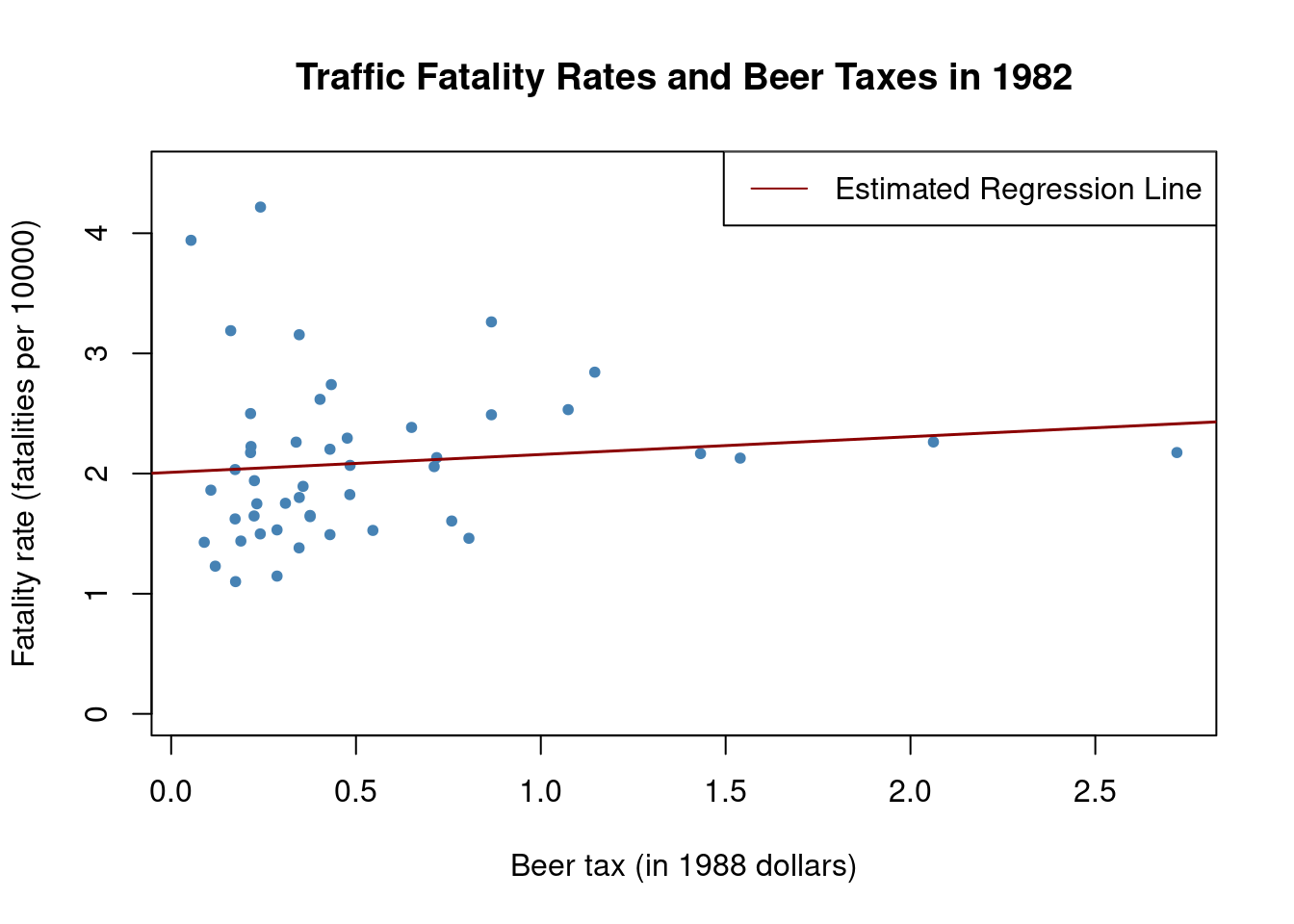
# plot observations and add estimated regression line for 1988 data
plot(x = as.double(Fatalities1988$beertax), y = as.double(Fatalities1988$fatal_rate),
     xlab = "Beer tax (in 1988 dollars)", ylab = "Fatality rate (fatalities per 10000)",
     main = "Traffic Fatality Rates and Beer Taxes in 1988", ylim = c(0, 4.5),
     pch = 20, col = "steelblue")

abline(fatal1988_mod, lwd = 1.5,col="darkred") # add the regression line to plot
legend("bottomright",lty=1,col="darkred","Estimated Regression Line") # add legend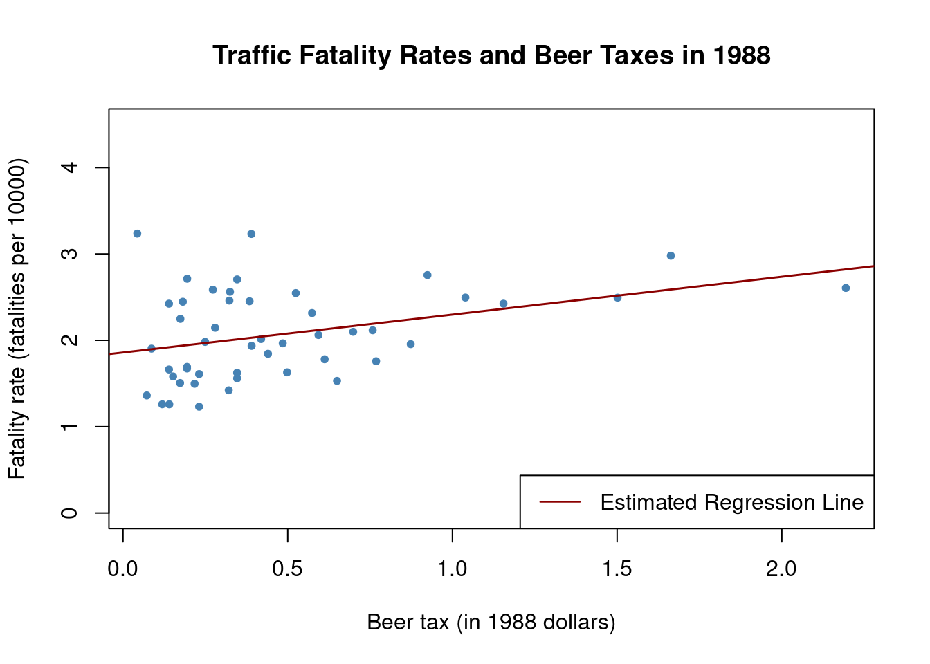
In both plots, each point represents observations of beer tax and fatality rate for a given state in the respective year. The regression results indicate a positive relationship between the beer tax and the fatality rate for both years.
The estimated coefficient on beer tax for the 1988 data is almost three times as large as for the 1982 dataset. This is contrary to our expectations: alcohol taxes are supposed to lower the rate of traffic fatalities. This is possibly due to omitted variable bias, since none of the models include any covariates, e.g., economic conditions.
This could be corrected for using a multiple regression approach. However, this cannot account for omitted unobservable factors that differ from state to state but can be assumed to be constant over the observation span, e.g., the populations’ attitude towards drunk driving. As shown in the next section, panel data allow us to hold such factors constant.
2.2 Two Time Periods: “Before and After” Comparisons
Let’s suppose there are only T=2 time periods t=1982,1988. This allows us to analyze differences in changes of the fatality rate from year 1982 to 1988. We start by considering the population regression model:
\text{FatalityRate}_{it} = \beta_0 + \beta_1 \text{BeerTax}_{it} + \beta_2 Z_i + u_{it}
where the Z_i are state specific characteristics that differ between states but are constant over time. For t=1982 and t=1988 we have
\begin{align*} FatalityRate_{i,1982} = \beta_0 + \beta_1 \text{BeerTax}_{i,1982} + \beta_2 Z_i + u_{i,1982}, \\ FatalityRate_{i,1988} = \beta_0 + \beta_1 \text{BeerTax}_{i,1988} + \beta_2 Z_i + u_{i,1988}. \end{align*}
We can eliminate the Z_i by regressing the difference in the fatality rate between 1988 and 1982 on the difference in beer tax between those years:
\text{FatalityRate}_{i,1988} - \text{FatalityRate}_{i,1982} = \beta_1 (\text{BeerTax}_{i,1988} - \text{BeerTax}_{i,1982}) + u_{i,1988} - u_{i,1982}
This regression model, where the difference in fatality rate between 1988 and 1982 is regressed on the difference in beer tax between those years, yields an estimate for \beta_1 that is robust to a possible bias due to omission of Z_i, as these influences are eliminated from the model. Next we will estimate a regression based on the differenced data and plot the estimated regression function.
# compute the differences
diff_fatal_rate <- Fatalities1988$fatal_rate - Fatalities1982$fatal_rate
diff_beertax <- Fatalities1988$beertax - Fatalities1982$beertax

# estimate a regression using differenced data
fatal_diff_mod <- lm(diff_fatal_rate ~ diff_beertax)
coeftest(fatal_diff_mod, vcov = vcovHC, type = "HC1")
t test of coefficients:

              Estimate Std. Error t value Pr(>|t|)
(Intercept)  -0.072037   0.065355 -1.1022 0.276091
diff_beertax -1.040973   0.355006 -2.9323 0.005229 **
---
Signif. codes:  0 '***' 0.001 '**' 0.01 '*' 0.05 '.' 0.1 ' ' 1
Including the intercept allows for a change in the mean fatality rate in the time between 1982 and 1988 in the absence of a change in the beer tax.
We obtain the OLS estimated regression function
\widehat{FatalityRate_{i1988} - FatalityRate_{i1982}} = \underset{(-0.065)}{0.072} - \underset{(0.36)}{1.04} \, (BeerTax_{i1988} - BeerTax_{i1982})
# plot the differenced data
plot(x = as.double(diff_beertax), y = as.double(diff_fatal_rate),
     xlab = "Change in beer tax (in 1988 dollars)",ylab = "Change in fatality rate (fatalities per 10000)",
     main = "Changes in Traffic Fatality Rates and Beer Taxes in 1982-1988", cex.main=1,
     xlim = c(-0.6, 0.6), ylim = c(-1.5, 1), pch = 20, col = "steelblue")

abline(fatal_diff_mod, lwd = 1.5,col="darkred") # add the regression line to plot
legend("topright",lty=1,col="darkred","Estimated Regression Line") #add legend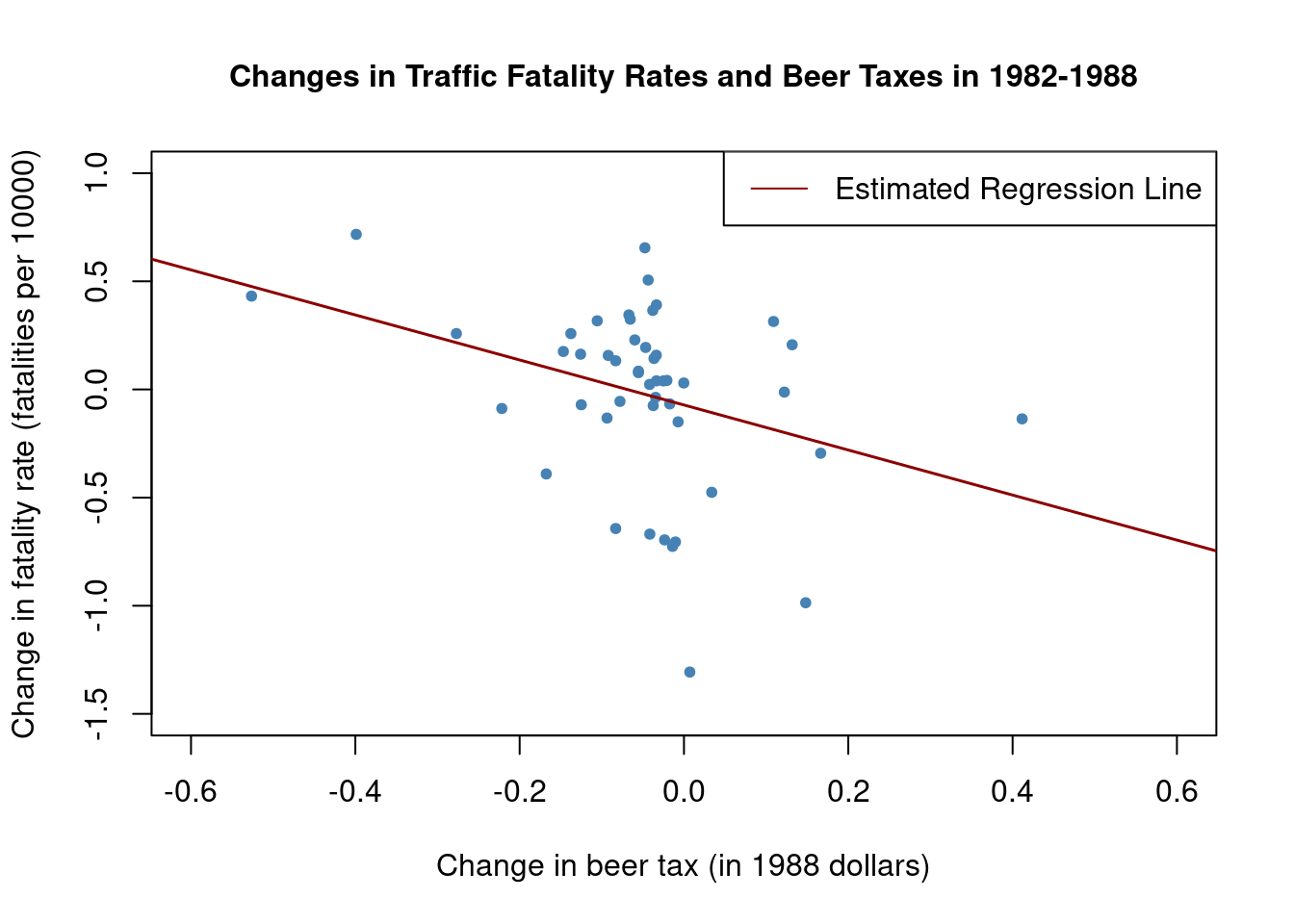
The estimated coefficient on beer tax is now negative and significantly different from zero at the 1\% significance level. Its interpretation is that raising the beer tax by \$1 is associated with an average decrease of 1.04 fatalities per 10,000 inhabitants. This is rather large as the average fatality rate is approximately 2 persons per 10,000 inhabitants.
# compute mean fatality rate over all states for all time periods
mean(Fatalities$fatal_rate)
[1] 2.040444The outcome we obtained is likely to be a consequence of omitting factors in the single-year regression that influence the fatality rate and are correlated with the beer tax and change over time. The message is that we need to be more careful and control for such factors before drawing conclusions about the effect of a raise in beer taxes.
The approach presented in this section discards information for years 1983 to 1987. The fixed effects method allows us to use data for more than T=2 time periods and enables us to add control variables to the analysis.
2.3 Fixed Effects Regression
Consider the panel regression model:
Y_{it} = \beta_0 + \beta_1 X_{it} + \beta_2 Z_i + u_{it} \tag{3.1} where the Z_i are unobserved time-invariant heterogeneities across the entities i = 1, \ldots, n. We aim to estimate \beta_1, the effect on Y_i of a change in X_i, holding constant Z_i. Letting \alpha_i = \beta_0 + \beta_2 Z_i, we obtain the model
Y_{it} = \alpha_i + \beta_1 X_{it} + u_{it} \tag{3.2} Having individual specific intercepts \alpha_i, i = 1, \ldots, n , where each of these can be understood as the fixed effect of entity i.
The Fixed Effects Regression Model is
Y_{it} = \beta_1 X_{1,it} + \cdots + \beta_k X_{k,it} + \alpha_i + u_{it} \tag{3.3}
with i = 1, \ldots, n and t = 1, \ldots, T. The \alpha_i are entity-specific intercepts that capture heterogeneities across entities. An equivalent representation of this model is given by
Y_{it} = \beta_0 + \beta_1 X_{1,it} + \cdots + \beta_k X_{k,it} + \gamma_2 D_{2i} + \gamma_3 D_{3i} + \cdots + \gamma_n D_{ni} + u_{it} \tag{3.4}
where the D_{2i}, D_{3i}, \ldots, D_{ni} are dummy variables.
To estimate the relation between traffic fatality rates and beer taxes, the simple fixed effects model is
FatalityRate_{it} = \beta_1 BeerTax_{it} + StateFixedEffects + u_{it} \tag{3.5}
a regression of the traffic fatality rate on beer tax and 48 binary regressors (one for each federal state). In this model, we are using a fixed effects approach to account for the effect of each federal state. Including a fixed effect for each state means that we’re estimating separate intercepts (or constant terms) for each state.
In R, we can simply use the function lm() to obtain an estimate of \beta_1.
fatal_fe_lm_mod <- lm(fatal_rate ~ beertax + state - 1, data = Fatalities)The -1 term tells R to exclude the intercept term that it would normally include by default. By doing this, we’re essentially saying that we don’t want to estimate an overall intercept for the model because we are already capturing the state-specific effects. This is a common practice in fixed effects models to avoid multicollinearity between the state-specific intercepts and the predictors.
summary(fatal_fe_lm_mod)It is also possible to estimate \beta_1 by applying OLS to the demeaned data, that is, to run the regression
\widetilde{FatalityRate} = \beta_1 \widetilde{BeertTax_{it}} + u_{it}
# obtain demeaned data
fatal_demeaned <- with(Fatalities,
            data.frame(fatal_rate = fatal_rate - ave(fatal_rate, state),
            beertax = beertax - ave(beertax, state)))

# estimate the regression
summary(lm(fatal_rate ~ beertax - 1, data = fatal_demeaned))
Call:
lm(formula = fatal_rate ~ beertax - 1, data = fatal_demeaned)

Residuals:
     Min       1Q   Median       3Q      Max
-0.58696 -0.08284 -0.00127  0.07955  0.89780

Coefficients:
        Estimate Std. Error t value Pr(>|t|)
beertax  -0.6559     0.1739  -3.772 0.000191 ***
---
Signif. codes:  0 '***' 0.001 '**' 0.01 '*' 0.05 '.' 0.1 ' ' 1

Residual standard error: 0.1757 on 335 degrees of freedom
Multiple R-squared:  0.04074,   Adjusted R-squared:  0.03788
F-statistic: 14.23 on 1 and 335 DF,  p-value: 0.0001913
The function ave is convenient for computing group averages. We use it to obtain state specific averages of the fatality rate and the beer tax.
The estimated coefficient is again −0.6559. The estimated regression function is
\widehat{FatalityRate} = \underset{(0.17)}{-0.66} \, BeerTax + StateFixedEffects \tag{3.6}
The coefficient on BeerTax is negative and statistically significant at the 0,1\% level. Its interpretation is that raising the beer tax by \$1 is associated with an average decrease of 0.66 fatalities per 10,000 people in traffic fatalities, which is still pretty high.
Although including state fixed effects eliminates the risk of a bias due to omitted factors that vary across states but not over time, we suspect that there are other omitted variables that vary over time and thus cause a bias.
2.4 Time Fixed Effects
Controlling for variables that are constant across entities but vary over time can be done by including time fixed effects. If there are only time fixed effects, the fixed effects regression model becomes
Y_{it} = \beta_0 + \beta_1 X_{it} + \delta_2 B_{2t} + \cdots + \delta_T BT_t + u_{it}
where only T−1 dummies are included (B1 is omitted) since the model includes an intercept. This model eliminates omitted variable bias caused by excluding unobserved variables that evolve over time but are constant across entities.
In some applications it is meaningful to include both entity (state) and time fixed effects. The entity and time fixed effects model is
Y_{it} = \beta_0 + \beta_1 X_{it} + \gamma_2 D_{2i} + \cdots + \gamma_n DT_i + \delta_2 B2_t + \cdots + \delta_T BT_t + u_{it}
The combined model allows to eliminate bias from unobservables that change over time but are constant over entities and it controls for factors that differ across entities but are constant over time. Such models can be estimated using the OLS algorithm that is implemented in R.
Let’s estimate the combined entity and time fixed effects model of the relation between fatalities and beer tax,
FatalityRate_{it} = \beta_1 BeerTax_{it} + StateFixedEffects + TimeFixedEffects + u_{it}
It is straightforward to estimate this regression with lm(). We just have to adjust the formula argument by adding the additional regressor year for time fixed effects:
# estimate a combined time and entity fixed effects regression model
fatal_tefe_lm_mod <- lm(fatal_rate ~ beertax + state + year - 1, data = Fatalities)summary(fatal_tefe_lm_mod)Before discussing the outcomes we convince ourselves that state and year are of the class factor
# check the class of 'state' and 'year'
class(Fatalities$state)
[1] "pseries" "factor" class(Fatalities$year)[1] "pseries" "factor" The lm() functions converts factors into dummies automatically. Since we exclude the intercept by adding -1 to the right-hand side of the regression formula, lm() estimates coefficients for n+(T−1)=48+6=54 binary variables (6 year dummies and 48 state dummies).
The estimated regression function is
\widehat{FatalityRate} = \underset{(0.20)}{-0.64} \, BeerTax + StateEffects + TimeFixedEffects \tag{3.7}
The result is close to the estimated coefficient for the regression model including only entity fixed effects, which was -0.66. Unsurprisingly, the coefficient is less precisely estimated, as we observe a slightly superior standard deviation for this new coefficient of -0.64. Nevertheless, it is still significantly different from zero at 1\% level.
We conclude that the estimated relationship between traffic fatalities and the real beer tax is not affected by omitted variable bias due to factors that are constant either over time or across states.
2.5 Driving Laws and Economic Conditions
There are two major sources of omitted variable bias that are not accounted for by all of the models of the relation between traffic fatalities and beer taxes that we have considered so far: economic conditions and driving laws.
Fortunately, Fatalities has data on state-specific legal drinking age (drinkage), punishment (jail, service) and various economic indicators like unemployment rate (unemp) and per capita income (income). We may use these covariates to extend the preceding analysis.
These covariates are defined as follows:
-
unemp: a numeric variable stating the state specific unemployment rate. -
log(income): the logarithm of real per capita income (in 1988 dollars). -
miles: the state average miles per driver. -
drinkage: the state specific minimum legal drinking age. -
drinkagec: a discretized version ofdrinkagethat classifies states into four categories of minimal drinking age; 18, 19, 20, 21 and older. R denotes this as[18,19),[19,20),[20,21)and[21,22]. These categories are included as dummy regressors where[21,22]is chosen as the reference category. -
punish: a dummy variable with levels yes and no that measures if drunk driving is severely punished by mandatory jail time or mandatory community service (first conviction).
First, we define some relevant variables to include in our following regression models:
# discretize the minimum legal drinking age
Fatalities$drinkagec <- cut(Fatalities$drinkage, breaks = 18:22, include.lowest = TRUE, right = FALSE)

# set minimum drinking age [21, 22] to be the baseline level
Fatalities$drinkagec <- relevel(Fatalities$drinkagec, "[21,22]")

# mandatory jail or community service?
Fatalities$punish <- with(Fatalities, factor(jail == "yes" | service == "yes", labels = c("no", "yes")))

# the set of observations on all variables for 1982 and 1988
fatal_1982_1988 <- Fatalities[with(Fatalities, year == 1982 | year == 1988), ]
Next, we estimate six regression models using plm().
# estimate all seven models
fat_mod1 <- lm(fatal_rate ~ beertax, data = Fatalities)

fat_mod2 <- plm(fatal_rate ~ beertax + state, data = Fatalities)

fat_mod3 <- plm(fatal_rate ~ beertax + state + year,
                       index = c("state","year"), model = "within",
                       effect = "twoways", data = Fatalities)

fat_mod4 <- plm(fatal_rate ~ beertax + state + year + drinkagec
                       + punish + miles + unemp + log(income),
                       index = c("state", "year"), model = "within",
                       effect = "twoways", data = Fatalities)

fat_mod5 <- plm(fatal_rate ~ beertax + state + year + drinkagec
                       + punish + miles,
                       index = c("state", "year"), model = "within",
                       effect = "twoways", data = Fatalities)

fat_mod6 <- plm(fatal_rate ~ beertax + year + drinkage
                       + punish + miles + unemp + log(income),
                       index = c("state", "year"), model = "within",
                       effect = "twoways", data = Fatalities)
We use stargazer() to generate a comprehensive tabular presentation of the results.
#load stargazer package
library(stargazer)

# gather clustered standard errors in a list
rob_se <- list(sqrt(diag(vcovHC(fat_mod1, type = "HC1"))),
               sqrt(diag(vcovHC(fat_mod2, type = "HC1"))),
               sqrt(diag(vcovHC(fat_mod3, type = "HC1"))),
               sqrt(diag(vcovHC(fat_mod4, type = "HC1"))),
               sqrt(diag(vcovHC(fat_mod5, type = "HC1"))),
               sqrt(diag(vcovHC(fat_mod6, type = "HC1"))))

# generate the table
stargazer(fat_mod1, fat_mod2, fat_mod3, fat_mod4, fat_mod5, fat_mod6,
          se = rob_se,
          type="html",
          omit.stat = "f", df=FALSE)
<table style="text-align:center"><tr><td colspan="7" style="border-bottom: 1px solid black"></td></tr><tr><td style="text-align:left"></td><td colspan="6"><em>Dependent variable:</em></td></tr>
<tr><td></td><td colspan="6" style="border-bottom: 1px solid black"></td></tr>
<tr><td style="text-align:left"></td><td colspan="6">fatal_rate</td></tr>
<tr><td style="text-align:left"></td><td><em>OLS</em></td><td colspan="5"><em>panel</em></td></tr>
<tr><td style="text-align:left"></td><td><em></em></td><td colspan="5"><em>linear</em></td></tr>
<tr><td style="text-align:left"></td><td>(1)</td><td>(2)</td><td>(3)</td><td>(4)</td><td>(5)</td><td>(6)</td></tr>
<tr><td colspan="7" style="border-bottom: 1px solid black"></td></tr><tr><td style="text-align:left">beertax</td><td>0.365<sup>***</sup></td><td>-0.656<sup>**</sup></td><td>-0.640<sup>*</sup></td><td>-0.445</td><td>-0.690<sup>**</sup></td><td>-0.456</td></tr>
<tr><td style="text-align:left"></td><td>(0.053)</td><td>(0.289)</td><td>(0.350)</td><td>(0.291)</td><td>(0.345)</td><td>(0.301)</td></tr>
<tr><td style="text-align:left"></td><td></td><td></td><td></td><td></td><td></td><td></td></tr>
<tr><td style="text-align:left">drinkagec[18,19)</td><td></td><td></td><td></td><td>0.028</td><td>-0.010</td><td></td></tr>
<tr><td style="text-align:left"></td><td></td><td></td><td></td><td>(0.068)</td><td>(0.081)</td><td></td></tr>
<tr><td style="text-align:left"></td><td></td><td></td><td></td><td></td><td></td><td></td></tr>
<tr><td style="text-align:left">drinkagec[19,20)</td><td></td><td></td><td></td><td>-0.018</td><td>-0.076</td><td></td></tr>
<tr><td style="text-align:left"></td><td></td><td></td><td></td><td>(0.049)</td><td>(0.066)</td><td></td></tr>
<tr><td style="text-align:left"></td><td></td><td></td><td></td><td></td><td></td><td></td></tr>
<tr><td style="text-align:left">drinkagec[20,21)</td><td></td><td></td><td></td><td>0.032</td><td>-0.100<sup>*</sup></td><td></td></tr>
<tr><td style="text-align:left"></td><td></td><td></td><td></td><td>(0.050)</td><td>(0.055)</td><td></td></tr>
<tr><td style="text-align:left"></td><td></td><td></td><td></td><td></td><td></td><td></td></tr>
<tr><td style="text-align:left">drinkage</td><td></td><td></td><td></td><td></td><td></td><td>-0.002</td></tr>
<tr><td style="text-align:left"></td><td></td><td></td><td></td><td></td><td></td><td>(0.021)</td></tr>
<tr><td style="text-align:left"></td><td></td><td></td><td></td><td></td><td></td><td></td></tr>
<tr><td style="text-align:left">punishyes</td><td></td><td></td><td></td><td>0.038</td><td>0.085</td><td>0.039</td></tr>
<tr><td style="text-align:left"></td><td></td><td></td><td></td><td>(0.101)</td><td>(0.109)</td><td>(0.101)</td></tr>
<tr><td style="text-align:left"></td><td></td><td></td><td></td><td></td><td></td><td></td></tr>
<tr><td style="text-align:left">miles</td><td></td><td></td><td></td><td>0.00001</td><td>0.00002<sup>*</sup></td><td>0.00001</td></tr>
<tr><td style="text-align:left"></td><td></td><td></td><td></td><td>(0.00001)</td><td>(0.00001)</td><td>(0.00001)</td></tr>
<tr><td style="text-align:left"></td><td></td><td></td><td></td><td></td><td></td><td></td></tr>
<tr><td style="text-align:left">unemp</td><td></td><td></td><td></td><td>-0.063<sup>***</sup></td><td></td><td>-0.063<sup>***</sup></td></tr>
<tr><td style="text-align:left"></td><td></td><td></td><td></td><td>(0.013)</td><td></td><td>(0.013)</td></tr>
<tr><td style="text-align:left"></td><td></td><td></td><td></td><td></td><td></td><td></td></tr>
<tr><td style="text-align:left">log(income)</td><td></td><td></td><td></td><td>1.816<sup>***</sup></td><td></td><td>1.786<sup>***</sup></td></tr>
<tr><td style="text-align:left"></td><td></td><td></td><td></td><td>(0.624)</td><td></td><td>(0.631)</td></tr>
<tr><td style="text-align:left"></td><td></td><td></td><td></td><td></td><td></td><td></td></tr>
<tr><td style="text-align:left">Constant</td><td>1.853<sup>***</sup></td><td></td><td></td><td></td><td></td><td></td></tr>
<tr><td style="text-align:left"></td><td>(0.047)</td><td></td><td></td><td></td><td></td><td></td></tr>
<tr><td style="text-align:left"></td><td></td><td></td><td></td><td></td><td></td><td></td></tr>
<tr><td colspan="7" style="border-bottom: 1px solid black"></td></tr><tr><td style="text-align:left">Observations</td><td>336</td><td>336</td><td>336</td><td>335</td><td>335</td><td>335</td></tr>
<tr><td style="text-align:left">R<sup>2</sup></td><td>0.093</td><td>0.041</td><td>0.036</td><td>0.360</td><td>0.066</td><td>0.357</td></tr>
<tr><td style="text-align:left">Adjusted R<sup>2</sup></td><td>0.091</td><td>-0.120</td><td>-0.149</td><td>0.217</td><td>-0.134</td><td>0.219</td></tr>
<tr><td style="text-align:left">Residual Std. Error</td><td>0.544</td><td></td><td></td><td></td><td></td><td></td></tr>
<tr><td colspan="7" style="border-bottom: 1px solid black"></td></tr><tr><td style="text-align:left"><em>Note:</em></td><td colspan="6" style="text-align:right"><sup>*</sup>p<0.1; <sup>**</sup>p<0.05; <sup>***</sup>p<0.01</td></tr>
</table>
While columns 2 and 3 recap the results of regressions 3.6 and 3.7, column 1 presents an estimate of the coefficient of interest in the naive OLS regression of the fatality rate on beer tax without any fixed effects. There we obtain a positive estimate for the coefficient on beer tax that is likely to be upward biased.
The sign of the estimate changes as we extend the model by both entity and time fixed effects in models 2 and 3. Nonetheless, as discussed before, the magnitudes of both estimates may be too large.
The model specifications 4 to 6 include covariates that shall capture the effect of overall state economic conditions as well as the legal framework. Nevertheless, considering model 4 as the baseline specification including covariates, we observe four interesting results:
1. Including these covariates is not leading to a major reduction of the estimated effect of the beer tax. The coefficient is not significantly different from zero at the 10\% level, which means that it is considered imprecise.
2. According to this regression model, the minimum legal drinking age is not associated with an effect on traffic fatalities: none of the three dummy variables are significantly different from zero at any common level of significance. Moreover, an F-Test of the joint hypothesis that all three coefficients are zero does not reject the null hypothesis. The next code chunk shows how to test this hypothesis:
# test if legal drinking age has no explanatory power
linearHypothesis(fat_mod4,test = "F",
                 c("drinkagec[18,19)=0", "drinkagec[19,20)=0", "drinkagec[20,21)"),
                 vcov. = vcovHC, type = "HC1")
Linear hypothesis test
Hypothesis:
drinkagec[18,19) = 0
drinkagec[19,20) = 0
drinkagec[20,21) = 0
Model 1: restricted model
Model 2: fatal_rate ~ beertax + state + year + drinkagec + punish + miles +
unemp + log(income)
Note: Coefficient covariance matrix supplied.
Res.Df Df F Pr(>F)
1 276
2 273 3 0.3782 0.76883. There is no statistical evidence indicating an association between punishment for first offenders and drunk driving: the corresponding coefficient is not significant at the 10\% level.
4. The coefficients on the economic variables representing employment rate and income per capita indicate an statistically significant association between these and traffic fatalities. We can check that the employment rate and income per capita coefficients are jointly significant at the 0.1\% level.
# test if economic indicators have no explanatory power
linearHypothesis(fat_mod4, test = "F",
                 c("log(income)", "unemp"), vcov. = vcovHC, type = "HC1")
Linear hypothesis test
Hypothesis:
log(income) = 0
unemp = 0
Model 1: restricted model
Model 2: fatal_rate ~ beertax + state + year + drinkagec + punish + miles +
unemp + log(income)
Note: Coefficient covariance matrix supplied.
Res.Df Df F Pr(>F)
1 275
2 273 2 31.577 4.609e-13 ***
---
Signif. codes: 0 '***' 0.001 '**' 0.01 '*' 0.05 '.' 0.1 ' ' 1Model 5 omits the economic factors. The result supports the notion that economic indicators should remain in the model as the coefficient on beer tax is sensitive to the inclusion of the latter.
Results for model 6 show that the legal drinking age has little explanatory power and that the coefficient of interest is not sensitive to changes in the functional form of the relation between drinking age and traffic fatalities.
2.6 Summary
We have not found statistical evidence to state that severe punishments and an increase the minimum drinking age could lead to a reduction of traffic fatalities due to drunk driving.
Nonetheless, there seems to be a negative effect of alcohol taxes on traffic fatalities according to our model estimate, However, this estimate is not precise and cannot be interpreted as the causal effect of interest, as there still may be a bias.
The issue is that there may be omitted variables that differ across states and change over time, and this bias remains even though we use a panel approach that controls for entity specific and time invariant unobservables.
A powerful method that can be used if common panel regression approaches fail is instrumental variables regression, which we will see in the next chapters.