7 Basic Principles
7.1 The frequentist approach
Observations are generated by a data generating process
Probabilistic model: {X_i \choose Y_i} \sim F_{xy}(\theta)
For example F_{xy}(\theta) represents N(µ, Σ) (joint normal)
If the conditional distribution is linear in X, we have \mathbb E(Y_i|X_i) = \alpha + \beta X_i
where Proof
\begin{align*} \alpha &= \mathbb{E}(Y_i) - \beta\, \mathbb{E}(X_i) \\ \beta &= \frac{\mathbb{E}(X_iY_i) - \mathbb{E}(X_i)\mathbb{E}(Y_i)}{\mathbb{E}(X_i^2) - [\mathbb{E}(X_i)]^2} = \frac{cov(Y_i, X_i)}{var(X_i)} \end{align*}
The OLS estimator can be seen as replacing the population moments by the sample moments
The conditional expectation answers the question: What is the expected value of Y_i if we were able to fix X_i at some prespecified value X_i = x?
The parameters of interest \theta = (\alpha, \beta)' result as a function of the joint distribution of X_i and Y_i, that is,
\theta = t(X_i, Y_i)
where \hat{\theta} denotes the estimated analog based on the available sample
The accuracy of the estimate is measured by
\begin{align*} \text{bias} &= \mathbb{E}(\hat{\theta}) - \theta &\text{(systematic deviation)} \\ \text{var} &= \mathbb{E}\left\{\left[\hat{\theta} - \mathbb{E}(\theta)\right]^2\right\} &\text{(unsystematic deviation)} \\ \text{MSE} &= \mathbb{E}\left[(\hat{\theta} - \theta)^2\right] = \text{bias}^2 + \text{var} &\text{(total deviation)} \end{align*}
The frequentist notion refers to “an infinite sequence of future trials”.
7.1.1 Estimation principles
a) Plug-in principle Replace t(X_i, Y_i) by its sample analogs:
\begin{align*} s_{xy} &= \frac{1}{n}\sum_{i=1}^{n} (x_i - \bar{x})(y_i - \bar{y}) \\ s_x^2 &= \frac{1}{n}\sum_{i=1}^{n} (x_i - \bar{x})^2 \end{align*}
and compute the estimator as b = s_{xy} / s_x^2
This often yields “optimal” estimators, but not always Accurrency measures and hypothesis tests can be obtained from the bootstrap principle
b) Maximum Likelihood
Joint density:
f_{\theta}(X_i, Y_i) = f_{\theta_1}(Y_i|X_i) f_{\theta_2}(X_i)
Maximizing the log-likelihood function:
\ell(\theta|X_i, Y_i) = \log f (X_i, Y_i) = \color{blue}{\log f_{\theta_1} (Y_i|X_i)} \color{black}{ + \log f_{\theta_2} (X_i)}
if {\theta_1} is independent of {\theta_2} we may maximize the conditional log-likelihood function:
\ell_c(\theta_1|X_i, Y_i) = \log f_{\theta_1}(Y_i|X_i) where in a simple regression: \theta_1 = (\alpha, \beta, \sigma^2)
Problem: the (family of) distribution needs to be known
Often some “natural” distribution is supposed, e.g. normal (Gaussian) distribution
ML estimators have optimal properties: - ML estimators are (asymptotically) unbiased - ML estimators are (asymptotically) efficient - ML estimators are (asymptotically) normally distributed
7.1.2 Further properties of ML estimators
- Consistency of the ML estimator just requires: \color{blue}{E[D(\theta)] = 0} where
D(\theta) = \frac{\partial \ell(\theta)}{\partial \theta} If the likelihood is misspecified but this condition is nevertheless fulfilled, then the estimator is called “pseudo ML”
- For large N and correctly specified likelihood the covariance matrix can be estimated by the information matrix
\text{var}(\hat\theta) = \color{blue}{I(\theta)^{-1}} \quad \color{black}{\text{where}} \quad I(\theta) = -E \left[ \frac{\partial^2 \ell(\theta)}{\partial \theta \partial \theta'} \right] = E [D(\theta)D(\theta)']
where \theta may be replaced by a consistent estimator. Example
- For pseudo ML estimators the covariance matrix needs to be adjusted (“sandwich estimator”)
7.2 The Bayesian approach
Bayes’ theorem: Reorganizing p(y, \theta) = p(\theta)p(y|\theta) = p(y)p(\theta|y) we obtain:
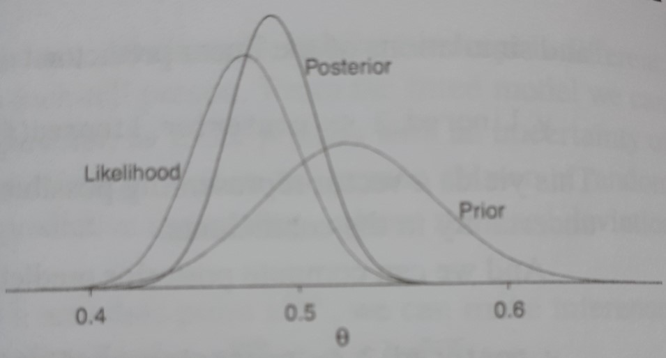
\underbrace{p(\theta|y)}_{\color{blue}{\text{posterior dis.}}} = \underbrace{p(\theta)}_{\color{red}{\text{prior dist.}}} \cdot \underbrace{\frac{L(\theta)}{p(y)}}_{\text{updating factor}} \\ \propto p(\theta) L(\theta) \quad (\propto \text{ : proportional to})
where L(\theta) = p(y|\theta) denotes the likelihood function
Bayesians prefer employing a conjugate family of distribution where the prior and posterior distribution are special cases of the same family of distributions
Example: y_i \sim \mathcal{N}(\mu, \sigma^2), where \sigma^2 is treated as known
\color{blue}{\text{prior distribution}} \color{black}{ \quad \mu \sim \mathcal{N}(\mu_0, \sigma_0^2) } This results in the posterior distribution:
\mu | y_1, \ldots, y_n \sim \mathcal{N}(\bar{\mu}, \bar{\sigma}^2) with
\bar{\mu} = \frac{1}{\psi_0 + \psi_1} (\psi_0 \mu_0 + \psi_1 Y) \quad\quad\quad \bar{\sigma}^2 = \frac{1}{\psi_0 + \psi_1}
\psi_0 = \frac{1}{\sigma_0^2} and \psi_1 = \frac{n}{\sigma^2} (precision)
7.2.1 Parameter Estimation
The MSE optimal estimate is obtained as
\hat\theta = E(\theta|y)
relationship to maximum likelihood:
\log p(\theta|y) = \text{const} + \underbrace{\log p(\theta)}_{O(1)} + \underbrace{\color{red}{\log L(\theta)}}_{O(N)} \Rightarrow as N \rightarrow \infty the mode of the posterior converge to ML
in most cases the posterior distribution is too difficult to be obtained analytically \Rightarrow Monte Carlo methods (Gibb sampler, MCMC simulator etc.)
Uniformative priors: Laplace’s principle of insufficient reason \Rightarrow uniform distribution (flat prior)
Uniform distribution does not need to be uninformative (parameter transformation, e.g. \psi = e^\theta)
Jeffreys’ prior is proportional to 1/\sigma_\theta (or square root of the Fisher information). Uniform prior is uninformative whenever \sigma_\theta does not depend on unknown parameters.
7.2.2 Comparison with the frequentist approach
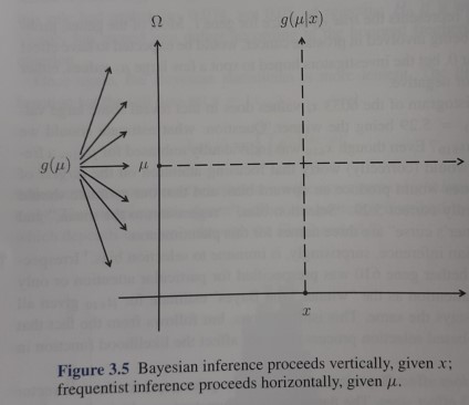
Bayesian approach takes care of knowledge accumulation
Bayesian machinery (MCMC) used to estimate extremely complicated models (frequentist approach fails)
Frequentist methods provide criteria for accessing the validity of the model. No such criteria for a Bayesian framework
7.3 Machine Learning Approach
Characteristics of the MLearn approach:
Big data. The data sets typically cover a large number of observations (nominal/qualitative, ordinal, metric). Large dimensional: many variables potentially useful for prediction
Algorithmic approach: The data is typically unstructured with no specific “data generating model”. Algorithms are constructed to learn the structure from the data
Limited theory. The algorithms are flexible and “trained” (instead of estimated) by the data. Avoiding overfitting by splitting data into training and test sets
MLern approaches are designed to cope with nonlinear data features
Consider the conditional mean function:
y_i = \color{red}{m(x_i)} \color{black}{ + u_i} where x_i is high dimensional (K may be even larger than N) and the functional form of m(\cdot) is unknown. The goal is to minimize
MSE = E\left[y_i - m(x_i)\right]^2
Supervised learning. Develop prediction rules for y_i given the vector x_i
Unsupervised learning. Uncovering structure amongst high-dimensional x_i
Classification. Assigning observations to groups (classes).
Sparsity. Finding out which variables can be ignored.
Computational Feasibility
Algorithmic learning requires powerful computational tools
Extensive packages in R and Python
An input produces some output. In between a black box. The (relative) performance is often not clear
“causal machine learning” tries to circumvent the correlation-is-not-causality critique
7.3.1 Regression as conditional expectation
Assume that the conditional expectation is a linear function such that
E(Y_i|X_i) = \alpha + \beta X_i Taking expectations with respect to X_i yields
\alpha = E(Y_i) - \beta E(X_i) Furthermore we have
\begin{align*} E(X_i Y_i) &= \underset{x}{E} [X_i E(Y_i|X_i)] = \alpha E(X_i) + \beta E(X_i^2) \\ E(X_i) E(Y_i) &= E(X_i) \underset{x}{E} [E(Y_i|X_i)] = \alpha E(X_i) + \beta [E(X_i)]^2 \end{align*}
Inserting the expression for \alpha yields
\beta = \frac{E(X_i Y_i) - E(X_i) E(Y_i)}{E(X_i^2) - [E(X_i)]^2} = \frac{\text{cov}(Y_i, X_i)}{\text{var}(X_i)} Back
7.3.2 ML estimation for the waiting time
Assume that the waiting time \tau_i is exponentially distributed with
\tau_i \sim \lambda e^{-\lambda \tau} \quad E(\tau_i) = \frac{1}{\lambda} \quad \text{var}(\tau_i) = \frac{1}{\lambda^2}
The log-likelihood function results as
\ell(\lambda) = N \log(\lambda) - \lambda \sum_{i=1}^{N} \tau_i with derivative
\frac{\partial \ell(\lambda)}{\partial \lambda} = \frac{N}{\lambda} - \sum_{i=1}^{N} \tau_i The ML estimator results as \hat\lambda = 1/\hat\tau . The information (matrix) results as
I(\lambda) = -E \left( -\frac{N}{\lambda^2} \right) = \frac{N}{\lambda^2} yielding var(\hat\lambda) = \lambda^2/N
The joint density results as
\begin{align*} \log L(X, \mu) + \log p(\mu) &= \text{const} - \frac{1}{2\sigma^2} \sum_{i=1}^{N} (Y_i - \mu)^2 - \underbrace{\frac{1}{2\sigma_0^2} (\mu - \mu_0)^2}_{\text{prior distribution}} \\ &= \text{const} - \underbrace{\frac{\psi_1 + \psi_0}{2}}_{1/(2 \bar{\sigma}^2)} \mu^2 + 2\mu \underbrace{\left( \frac{\psi_1 \bar{Y} + \psi_0 \mu_0}{2} \right)}_{\bar{\mu}/(2 \bar{\sigma}^2)} + \dots \end{align*}
such that
\begin{align*} \bar{\sigma}^2 &= \frac{1}{\psi_1 + \psi_0} = \frac{1}{(n/\sigma^2) + (1/\sigma_0^2)} \\ \bar{\mu} &= \frac{1}{\psi_1 + \psi_0}(\psi_1\bar{Y} + \psi_0\mu_0) \end{align*}