9 Machine Learning Methods
OLS regression requires sufficient degrees of freedom (N-K)
Asymptotic theory assumes N - K \rightarrow \infty
Standard asymptotic results are invalid if K/N \rightarrow \kappa > 0
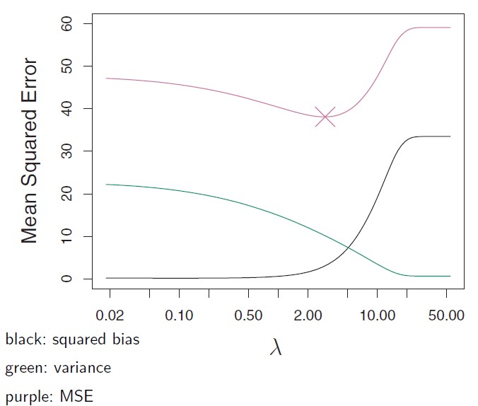
OLS estimation typically no/small bias but large variance
Performance is measured by the “risk”, typically mean-squared error:
E(b - \beta)^2 = \color{blue}{ \underbrace{ E\left\{[b - E(b)]^2 \right\}}_{\text{variance}} } \color{black}{+} \color{red}{ \underbrace{[E(b) - \beta]^2}_{\text{bias}^2} }
The variance represents the unsystematic error and the bias the systematic error. If the parameters are estimated only oncy, the distinction becomes irrelevant.
Ridge estimation
Introducing an L_2 penalty: S^R_\lambda = (y - X\beta)^\prime(y - X\beta) + \lambda \|\beta\|^2 where \|\beta\| = \sqrt{\sum_{j=1}^{K} \beta_j^2} denotes the Gaussian norm
minimizing S^R_\lambda yields the Ridge estimator
\widehat\beta_R = \left(X'X + \lambda I_K\right)^{-1}X'y
If K > N then X'X is singular but X'X + \lambda I_K is not!
Since X'X + \lambda I_K is “larger” than X'X (in a matrix sense) the coefficients in \widehat\beta_R “shrink towards zero” as \lambda gets large
Choice of \lambda is typically data driven (see below)
9.1 Lasso Regression
“Sparse regression”: Many of the coefficients are actually zero
Define the L_r norm as
\|\beta\|_r = \left( \sum_{j=1}^{K} |\beta_j|^r \right)^{1/r}
such that
S^L_\lambda = (y - X\beta)^\prime(y - X\beta) + \lambda \|\beta\|_1
L_1 penalty corresponds to the constraint:
\sum_{j=1}^{K} |\beta_j| \leq \tau
Solution of the minimization problem by means of quadratic programming
The solution typically involves zero coefficients
Some more details
The regressors and dependent variables are typically standardized:
\tilde{x}_{j,i} = (x_{j,i} - \bar{x}_j) / s_j where \bar{x}_j and s_j are the mean and standard deviation of x_j
Relationship to pre-test estimator: For a simple regression The first order condition is given by:
\begin{align*} \frac{2}{N} \left( \sum_{i=1}^{N} \tilde{x}_i \tilde{y}_i - \frac{\lambda}{N} \sum_{i=1}^{N} \tilde{x}_i^2 \beta \right) \pm \lambda &\stackrel{!}{=} 0 \\ \beta - \widehat\beta^L_\lambda \pm \frac{N}{2} \lambda &\stackrel{!}{=} 0 \end{align*}
and therefore:
\widehat\beta^L_\lambda = \begin{cases} b + \lambda^* & \text{if } b < -\lambda^* \\ 0 & \text{if } -\lambda^* \leq b \leq \lambda^* \\ b - \lambda^* & \text{if } b > \lambda^* \end{cases} where \lambda^* = \lambda \cdot N/2
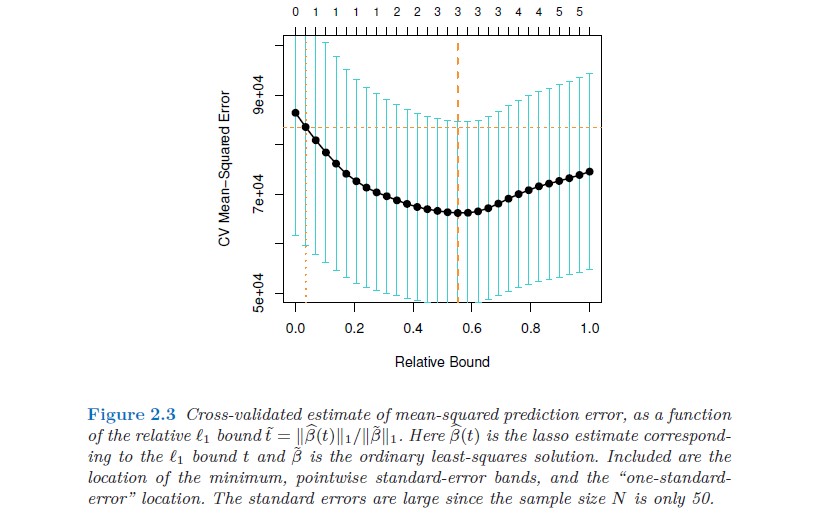
Selecting the shrinkage parameter
Trade-off between bias (large \lambda) and variance (small \lambda).
Choose \lambda that minimizes the MSE = Bias^2 + Var
leave-one-out cross validation:
Drop one observation and forecast it based on the remaining N-1 observations
k-fold cross validation:
divide randomly the set of observations into k groups (folds) of approximately equal size. The first fold is treated as a validation set and the remaining k-1 folds are employed for parameter estimation
evaluate the loss (MSE) for each observation conditional on \lambda and compute the average loss as a function of \lambda
Minimize the loss (MSE) with respect to \lambda
k is typically between 5 - 10
Refinements
post-Lasso estimation: Re-estimate the parameters by OLS leaving out the coefficients that were set to zero by LASSO
oracle property: the asymptotic distribution of the estimator is the same as if we knew which coefficient is equal to zero
Original LASSO does not exhibit the oracle property
Adaptive LASSO: with weighted penalty \sum_{j=1}^{K} \widehat w_j |\beta_j| and \widehat w_j = 1/| b_j|^{\nu} \quad \quad \text{with some } v > 0 where b_j denotes the OLS estimate
if K > N replace b_j by the simple regression coefficient
Adaptive LASSO possesses the oracle property
Elastic net: hybrid method LASSO/Ridge
S^L_\lambda = (y - X\beta)^\prime \,(y - X\beta) + \lambda_1 \, \|\beta\|_1 \,+ \,\lambda_2 \,\|\beta\|_2^2
9.2 Dimension reduction techniques
if k is large, it is desirable to reduce the dimensionality by using linear combinations
Z_m = \sum_{j=1}^{k} \phi_{jm}X_j \quad \quad m = 1, \ldots, k
where \phi_{1m}, \ldots ,\phi_{km} as unknown constants such that M << k
Using these linear combinations (“common factors”, principal components) the regression becomes
y_i = \theta_0 + \sum_{m=1}^{M} \theta_m z_{im} + \epsilon_i
Inserting shows that the elements of \beta fulfills the restriction
\beta_j = \sum_{m=1}^{M} \theta_m \phi_{jm}
choose \phi_{1m}, \ldots ,\phi_{km} such that the “loss of information” is minimal
Principal component regression
choose the linear combinations Z_m such that they explain most of X_j:
X_j = \sum_{m=1}^{M} \alpha_{jm} Z_m + v_j such that the variance of v_j is minimized:
S^2(\alpha, \phi) = \sum_{j=1}^{k} \sum_{i=1}^{n} v_{ji}^2
The linear combination is obtained from the eigenvectors of the sample covariance matrix of X
The number of linear combinations, M, can be determined by considering the ordered eigenvalues
Another approach is the method of Partial Least-Squares, where the linear combinations are found sequentially by considering the covariance with the dependent variable
Computational Details
let X denote an N \times K matrix of regressors, then
X = ZA' + V where Z is N \times M where M < K. Inserting in the model for y yields
\begin{align*} y &= Z\underbrace{A'\beta} + \underbrace{u + V\beta} \\ &= \quad Z'\theta \; + \quad \epsilon \end{align*}
the estimates can be obtained from the “singular value decomposition”:
\begin{align*} X &= UDV' \\ \text{where} \quad U'U &= I_N \quad \text{and} \quad V'V = I_k \end{align*}
and D an N \times K diagonal matrix of the K singular values
the dimension reduction is obtained by dropping the last N - M and K - M columns of U and V respectively.
the matrix Z (loading matrix) is obtained as \color{red}{U_M} and \color{blue}{F = D_M V'_M} is the matrix of factors
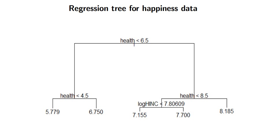
9.3 Regression trees / Random forest
piecewise constant function:
f(x) = \sum_{j=1}^{J} \mathbf{1}(x \in R_j)c_j
where R_j = [s_{j-1},s_j) is some region in the real space
finding the best split point s for some splitting variable x_{j,i} is simple if there are only two regions (J = 2) such that
\min_s \left[ \sum_{i \in R_1} (y_i - \widehat c_1)^2 + \sum_{i \in R_2} (y_i - \widehat c_2)^2 \right]
we can proceed by searching for the next optimal split in the regions R_1 and R_2 and so on
how far do we need to extend this tree? Typically we stop if the region becomes dense (node size < 5, say)
Pruning the tree: Keep only the branches that result in a sufficient (involving some parameter \alpha) reduction of the objective function. \alpha is chosen by cross validation.
Bagging: Full sample Z = \{ (x'_1, y_1), (x'_2, y_2), \ldots, (x'_N, y_N) \}
The bootstrap sample: is obtained by drawing randomly from the set {1, 2, \cdots, N} such that Z^*_b = \{ (x_1^{*\prime}, y_1^*), (x_2^{*\prime}, y_2^*), \ldots, (x_N^{*\prime}, y_N^*) \} Let \widehat f_b^*(x) denote the prediction based on the regression fit based on Z^*_b. The aggregated prediction is obtained as
\hat f_{\text{bag}}(x) = \frac{1}{B} \sum_{b=1}^{B} \widehat f^*_{b}(x)
Bootstrap aggregation stabilizes the unstable outcome of a regression tree
Specifically, when growing a tree on a bootstrapped dataset: Before each split, select m < p, e.g. m = int( \sqrt p) of the input variables at random as candidates for splitting.
This reduces the correlation among the bootstrap draws