5 Empirical Applications of Experiments
In this chapter, we explore statistical techniques frequently used to quantify the causal impacts of programs, policies, or interventions. Statisticians advocate for an optimal research design known as an ideal randomized controlled experiment, which involves randomly allocating subjects into two distinct groups: a treatment group receiving the intervention and a control group not receiving it. By comparing outcomes between these groups, researchers can estimate the average treatment effect.
We will make use of the following packages in R:
AER (Christian Kleiber and Zeileis 2008)
dplyr (Wickham et al. 2023)
MASS (Ripley 2023)
mvtnorm (Genz et al. 2023)
rddtools (Stigler and Quast 2022)
scales (Wickham and Seidel 2022)
stargazer(Hlavac 2022)
tidyr (Wickham, Vaughan, and Girlich 2023)
6 Experiments
6.1 Data Set Description & Experimental Design
The Project Student-Teacher Achievement Ratio (STAR) was a large-scale randomized controlled experiment aimed at determining the effectiveness of class size reduction in improving elementary education.
This 4-year experiment took place during the 1980s in 80 elementary schools across Tennessee by the State Department of Education.
During the initial year, approximately 6,400 students were randomly allocated to one of three interventions:
Treatment 1: small class (13 to 17 students per teacher).
Treatment 2: regular-with-aide class (22 to 25 students with a full-time teacher’s aide).
Control group: regular class (22 to 25 students per teacher).
Additionally, teachers were randomly assigned to the classes they taught. These interventions started as students entered kindergarten and continued until third grade.
The students’ academic evolution was evaluated by aggregating the scores achieved on both the math and reading sections of the Stanford Achievement Test.
Let’s start loading the STAR data set from the AER package and exploring it
     gender ethnicity   birth stark star1 star2   star3 readk read1 read2 read3
1122 female      afam 1979 Q3  <NA>  <NA>  <NA> regular    NA    NA    NA   580
1137 female      cauc 1980 Q1 small small small   small   447   507   568   587
     mathk math1 math2 math3   lunchk lunch1   lunch2 lunch3 schoolk school1
1122    NA    NA    NA   564     <NA>   <NA>     <NA>   free    <NA>    <NA>
1137   473   538   579   593 non-free   free non-free   free   rural   rural
     school2  school3  degreek  degree1  degree2  degree3 ladderk ladder1
1122    <NA> suburban     <NA>     <NA>     <NA> bachelor    <NA>    <NA>
1137   rural    rural bachelor bachelor bachelor bachelor  level1  level1
        ladder2    ladder3 experiencek experience1 experience2 experience3
1122       <NA>     level1          NA          NA          NA          30
1137 apprentice apprentice           7           7           3           1
     tethnicityk tethnicity1 tethnicity2 tethnicity3 systemk system1 system2
1122        <NA>        <NA>        <NA>        cauc    <NA>    <NA>    <NA>
1137        cauc        cauc        cauc        cauc      30      30      30
     system3 schoolidk schoolid1 schoolid2 schoolid3
1122      22      <NA>      <NA>      <NA>        54
1137 30 63 63 63 63dim(STAR)[1] 11598 47# get variable names
names(STAR) [1] "gender" "ethnicity" "birth" "stark" "star1"
[6] "star2" "star3" "readk" "read1" "read2"
[11] "read3" "mathk" "math1" "math2" "math3"
[16] "lunchk" "lunch1" "lunch2" "lunch3" "schoolk"
[21] "school1" "school2" "school3" "degreek" "degree1"
[26] "degree2" "degree3" "ladderk" "ladder1" "ladder2"
[31] "ladder3" "experiencek" "experience1" "experience2" "experience3"
[36] "tethnicityk" "tethnicity1" "tethnicity2" "tethnicity3" "systemk"
[41] "system1" "system2" "system3" "schoolidk" "schoolid1"
[46] "schoolid2" "schoolid3" We observe a variety of factor variables describing student and teacher characteristics, as well as several school indicators recorded for each of the four academic years.
The data set contains a total of 11598 observations on 47 variables and it is presented in what is called a wide format, that is, each column represents a variable and each student is represented by a row, where the values for each variable are recorded.
We see that most of the variable names end with a suffix (k, 1, 2, 3) which correspond to the grade for which the value of the variable was registered. This allows adjusting the formula argument in lm() for each grade by simply changing the variables’ suffixes accordingly.
From the output of head(STAR, 2) we observe some missing values as NA. This is because the student entered the experiment in the third grade in a regular class.
Consequently, the class size is documented in star3, while the other class type indicator variables are marked as NA. The student’s math and reading scores for the third grade are provided, while data for other grades are absent for the same reason.
To obtain only her non-missing recordings, we can easily remove the NAs using the !is.na() function.
# drop NA recordings for the first observation and print to the console
STAR[1, !is.na(STAR[1, ])]
gender ethnicity birth star3 read3 math3 lunch3 school3 degree3
1122 female afam 1979 Q3 regular 580 564 free suburban bachelor
ladder3 experience3 tethnicity3 system3 schoolid3
1122 level1 30 cauc 22 54is.na(STAR[1, ]) returns a logical vector with TRUE at positions that correspond to missing entries for the first observation. By using the ! operator, we invert the result to obtain only non-NA entries for the first student in the data set.
When using lm(), it is not necessary to remove rows with missing data, as it is done by default. Removing missing data might lead to a small number of observations, which can make our estimates less accurate and our conclusions unreliable.
However, this isn’t a problem in our study because, as we’ll see later, we have more than 5000 observations for each of the regressions we will conduct.
6.2 Analysis of the STAR data
Because there are two treatment groups (small class and regular-sized class with an aide), the regression version of the differences estimator requires adjustment to accommodate these groups along with the control group.
This adjustment involves introducing two binary variables: one indicating whether the student is in a small class and another indicating whether the student is in a regular-sized class with an aide. This leads to the population regression model
Y_i=\beta_0+\beta_1 \, SmallClass_i + \beta_2 \, RegAide_i + u_i \tag{6.1}
where Y_i represents a test score, SmallClass_i equals 1 if the i^{th} student is in a small class and 0 otherwise, and RegAide_i equals 1 if the i^{th} student is in a regular class with an aide and 0 otherwise.
The effect on the test score of being in a small class relative to a regular class is \beta_1, and the effect of being in a regular class with an aide relative to a regular class is \beta_2.
The differences estimator for the experiment can then be calculated by estimating \beta_1 and \beta_2 in Equation (6.1) using ordinary least squares (OLS).
We will now perform regression (6.1) for each grade separately. The dependent variable will be the sum of the points scored in the math and reading parts, which can be constructed using I().
# compute differences estimates for each grade
fmk <- lm(I(readk + mathk) ~ stark, data = STAR) # kindergarten
fm1 <- lm(I(read1 + math1) ~ star1, data = STAR) # first grade
fm2 <- lm(I(read2 + math2) ~ star2, data = STAR) # second grade
fm3 <- lm(I(read3 + math3) ~ star3, data = STAR) # third grade
# obtain coefficient matrix using robust standard errors
coeftest(fmk, vcov = vcovHC, type= "HC1")
t test of coefficients:

                   Estimate Std. Error  t value  Pr(>|t|)
(Intercept)       918.04289    1.63339 562.0473 < 2.2e-16 ***
starksmall         13.89899    2.45409   5.6636 1.554e-08 ***
starkregular+aide   0.31394    2.27098   0.1382    0.8901
---
Signif. codes: 0 '***' 0.001 '**' 0.01 '*' 0.05 '.' 0.1 ' ' 1coeftest(fm1, vcov = vcovHC, type= "HC1")
t test of coefficients:

                   Estimate Std. Error  t value  Pr(>|t|)
(Intercept)       1039.3926     1.7846 582.4321 < 2.2e-16 ***
star1small          29.7808     2.8311  10.5190 < 2.2e-16 ***
star1regular+aide   11.9587     2.6520   4.5093  6.62e-06 ***
---
Signif. codes: 0 '***' 0.001 '**' 0.01 '*' 0.05 '.' 0.1 ' ' 1coeftest(fm2, vcov = vcovHC, type= "HC1")
t test of coefficients:

                   Estimate Std. Error  t value  Pr(>|t|)
(Intercept)       1157.8066     1.8151 637.8820 < 2.2e-16 ***
star2small          19.3944     2.7117   7.1522  9.55e-13 ***
star2regular+aide    3.4791     2.5447   1.3672    0.1716
---
Signif. codes: 0 '***' 0.001 '**' 0.01 '*' 0.05 '.' 0.1 ' ' 1coeftest(fm3, vcov = vcovHC, type= "HC1")
t test of coefficients:

                    Estimate Std. Error  t value  Pr(>|t|)
(Intercept)       1228.50636    1.68001 731.2483 < 2.2e-16 ***
star3small          15.58660    2.39604   6.5051 8.393e-11 ***
star3regular+aide   -0.29094    2.27271  -0.1280    0.8981
---
Signif. codes:  0 '***' 0.001 '**' 0.01 '*' 0.05 '.' 0.1 ' ' 1
We can present as usual our results in a table using stargazer()
# compute robust standard errors for each model and gather them in a list
rob_se_1 <- list(sqrt(diag(vcovHC(fmk, type = "HC1"))),
                 sqrt(diag(vcovHC(fm1, type = "HC1"))),
                 sqrt(diag(vcovHC(fm2, type = "HC1"))),
                 sqrt(diag(vcovHC(fm3, type = "HC1"))))

stargazer(fmk,fm1,fm2,fm3,
  se = rob_se_1,
  type="html",
  omit.stat = "f", df=FALSE)
<table style="text-align:center"><tr><td colspan="5" style="border-bottom: 1px solid black"></td></tr><tr><td style="text-align:left"></td><td colspan="4"><em>Dependent variable:</em></td></tr>
<tr><td></td><td colspan="4" style="border-bottom: 1px solid black"></td></tr>
<tr><td style="text-align:left"></td><td>I(readk + mathk)</td><td>I(read1 + math1)</td><td>I(read2 + math2)</td><td>I(read3 + math3)</td></tr>
<tr><td style="text-align:left"></td><td>(1)</td><td>(2)</td><td>(3)</td><td>(4)</td></tr>
<tr><td colspan="5" style="border-bottom: 1px solid black"></td></tr><tr><td style="text-align:left">starksmall</td><td>13.899<sup>***</sup></td><td></td><td></td><td></td></tr>
<tr><td style="text-align:left"></td><td>(2.454)</td><td></td><td></td><td></td></tr>
<tr><td style="text-align:left"></td><td></td><td></td><td></td><td></td></tr>
<tr><td style="text-align:left">starkregular+aide</td><td>0.314</td><td></td><td></td><td></td></tr>
<tr><td style="text-align:left"></td><td>(2.271)</td><td></td><td></td><td></td></tr>
<tr><td style="text-align:left"></td><td></td><td></td><td></td><td></td></tr>
<tr><td style="text-align:left">star1small</td><td></td><td>29.781<sup>***</sup></td><td></td><td></td></tr>
<tr><td style="text-align:left"></td><td></td><td>(2.831)</td><td></td><td></td></tr>
<tr><td style="text-align:left"></td><td></td><td></td><td></td><td></td></tr>
<tr><td style="text-align:left">star1regular+aide</td><td></td><td>11.959<sup>***</sup></td><td></td><td></td></tr>
<tr><td style="text-align:left"></td><td></td><td>(2.652)</td><td></td><td></td></tr>
<tr><td style="text-align:left"></td><td></td><td></td><td></td><td></td></tr>
<tr><td style="text-align:left">star2small</td><td></td><td></td><td>19.394<sup>***</sup></td><td></td></tr>
<tr><td style="text-align:left"></td><td></td><td></td><td>(2.712)</td><td></td></tr>
<tr><td style="text-align:left"></td><td></td><td></td><td></td><td></td></tr>
<tr><td style="text-align:left">star2regular+aide</td><td></td><td></td><td>3.479</td><td></td></tr>
<tr><td style="text-align:left"></td><td></td><td></td><td>(2.545)</td><td></td></tr>
<tr><td style="text-align:left"></td><td></td><td></td><td></td><td></td></tr>
<tr><td style="text-align:left">star3small</td><td></td><td></td><td></td><td>15.587<sup>***</sup></td></tr>
<tr><td style="text-align:left"></td><td></td><td></td><td></td><td>(2.396)</td></tr>
<tr><td style="text-align:left"></td><td></td><td></td><td></td><td></td></tr>
<tr><td style="text-align:left">star3regular+aide</td><td></td><td></td><td></td><td>-0.291</td></tr>
<tr><td style="text-align:left"></td><td></td><td></td><td></td><td>(2.273)</td></tr>
<tr><td style="text-align:left"></td><td></td><td></td><td></td><td></td></tr>
<tr><td style="text-align:left">Constant</td><td>918.043<sup>***</sup></td><td>1,039.393<sup>***</sup></td><td>1,157.807<sup>***</sup></td><td>1,228.506<sup>***</sup></td></tr>
<tr><td style="text-align:left"></td><td>(1.633)</td><td>(1.785)</td><td>(1.815)</td><td>(1.680)</td></tr>
<tr><td style="text-align:left"></td><td></td><td></td><td></td><td></td></tr>
<tr><td colspan="5" style="border-bottom: 1px solid black"></td></tr><tr><td style="text-align:left">Observations</td><td>5,786</td><td>6,379</td><td>6,049</td><td>5,967</td></tr>
<tr><td style="text-align:left">R<sup>2</sup></td><td>0.007</td><td>0.017</td><td>0.009</td><td>0.010</td></tr>
<tr><td style="text-align:left">Adjusted R<sup>2</sup></td><td>0.007</td><td>0.017</td><td>0.009</td><td>0.010</td></tr>
<tr><td style="text-align:left">Residual Std. Error</td><td>73.490</td><td>90.501</td><td>83.694</td><td>72.910</td></tr>
<tr><td colspan="5" style="border-bottom: 1px solid black"></td></tr><tr><td style="text-align:left"><em>Note:</em></td><td colspan="4" style="text-align:right"><sup>*</sup>p<0.1; <sup>**</sup>p<0.05; <sup>***</sup>p<0.01</td></tr>
</table>
Based on the estimates, students in kindergarten seem to benefit significantly from being in smaller classes, showing an average test score increase of 13.9 points compared to those in regular classes.
However, the effect of having an aide in a regular class is minimal, with an estimated increase of only 0.31 points on the test.
Across all grades, the data indicates that smaller classes lead to improved test scores, rejecting the idea that they provide no benefit at a 1\% significance level.
Yet, the evidence for the effectiveness of having an aide in a regular class is less conclusive, except for first graders, even at a 10\% significance level.
The estimated improvements in smaller classes are similar across kindergarten, 2nd, and 3rd grades, though the effect appears slightly stronger in first grade.
Overall, the results suggest that reducing class size has a noticeable impact on test performance, whereas adding an aide to a regular-sized class has only a minor effect, possibly close to zero.
6.3 Including Additional Regressors
In our study case, there may be other variables that explain the variation in the dependent variable. For this reason, by adding additional regressors to the model, we can enhance the precision of the estimated causal effects.
The differences estimator with additional regressors is more efficient than the differences estimator if the additional regressors explain some of the variation in the dependent variable.
Moreover, if the treatment allocation was not completely random due to protocol deviations, our previous estimates could be biased.
To address these concerns and provide more robust estimates, we will now include additional regressors measuring teacher, school, and student characteristics, particularly focusing on kindergarten. We consider the following variables:
experience- Teacher’s years of experienceboy- Student is a boy (dummy)lunch- Free lunch eligibility (dummy)black- Student is African-American (dummy)race- Student’s race is other than black or white (dummy)schoolid- School indicator variables
We will use these extra regressors to estimate the following models:
\begin{align} Y_i &= \beta_0 + \beta_1 \, SmallClass_i + \beta_2 \, RegAide_i + u_i, &\tag{6.2} \\ Y_i &= \beta_0 + \beta_1 \, SmallClass_i + \beta_2 \, RegAide_i + \beta_3 \, experience_i + u_i, &\tag{6.3} \\ Y_i &= \beta_0 + \beta_1 \, SmallClass_i + \beta_2 \, RegAide_i + \beta_3 \, experience_i + \, schoolid + u_i, &\tag{6.4} \\ Y_i &= \beta_0 + \beta_1 \, SmallClass_i + \beta_2 \, RegAide_i + \beta_3 \, experience_i + \beta_4 \, boy + \beta_5 \, lunch \\ &\quad + \, \beta_6 \, black + \beta_7 \, race + schoolid + u_i. &\tag{6.5} \end{align}
With the help of functions from the dplyr and tidyr packages, we will create our custom subset of the data, including only kindergarten data.
First, we will use transmute() to keep only relevant variables (gender, ethnicity, stark, readk, mathk, lunchk, experiencek and schoolidk) and drop the rest.
Then, using mutate() and logical statements within the function ifelse(), we will add the additional binary variables black, race and boy.
To keep it short, we skip displaying the coefficients for the indicator dummies in the coeftest() output by subsetting the matrices.
# obtain robust inference on the significance of coefficients
coeftest(gradeK1, vcov. = vcovHC, type = "HC1")
t test of coefficients:

                   Estimate Std. Error  t value  Pr(>|t|)
(Intercept)       904.72124    2.22235 407.1020 < 2.2e-16 ***
starksmall         14.00613    2.44704   5.7237 1.095e-08 ***
starkregular+aide  -0.60058    2.25430  -0.2664    0.7899
experiencek         1.46903    0.16929   8.6778 < 2.2e-16 ***
---
Signif. codes: 0 '***' 0.001 '**' 0.01 '*' 0.05 '.' 0.1 ' ' 1coeftest(gradeK2, vcov. = vcovHC, type = "HC1")[1:4, ] Estimate Std. Error t value Pr(>|t|)
(Intercept) 925.6748750 7.6527218 120.9602155 0.000000e+00
starksmall 15.9330822 2.2411750 7.1092540 1.310324e-12
starkregular+aide 1.2151960 2.0353415 0.5970477 5.504993e-01
experiencek 0.7431059 0.1697619 4.3773429 1.222880e-05coeftest(gradeK3, vcov. = vcovHC, type = "HC1")[1:7, ] Estimate Std. Error t value Pr(>|t|)
(Intercept) 937.6831330 14.3726687 65.2407117 0.000000e+00
starksmall 15.8900507 2.1551817 7.3729516 1.908960e-13
starkregular+aide 1.7869378 1.9614592 0.9110247 3.623211e-01
experiencek 0.6627251 0.1659298 3.9940097 6.578846e-05
boy -12.0905123 1.6726331 -7.2284306 5.533119e-13
lunchkfree -34.7033021 1.9870366 -17.4648529 1.437931e-66
black -25.4305130 3.4986918 -7.2685776 4.125252e-13And we display the results in a stargazer() table
# compute robust standard errors for each model and gather them in a list
rob_se_2 <- list(sqrt(diag(vcovHC(fmk, type = "HC1"))),
                 sqrt(diag(vcovHC(gradeK1, type = "HC1"))),
                 sqrt(diag(vcovHC(gradeK2, type = "HC1"))),
                 sqrt(diag(vcovHC(gradeK3, type = "HC1"))))
stargazer(fmk, gradeK1, gradeK2, gradeK3,
          se = rob_se_2,
          type="html",
          omit.stat = "f", df=FALSE)
<table style="text-align:center"><tr><td colspan="5" style="border-bottom: 1px solid black"></td></tr><tr><td style="text-align:left"></td><td colspan="4"><em>Dependent variable:</em></td></tr>
<tr><td></td><td colspan="4" style="border-bottom: 1px solid black"></td></tr>
<tr><td style="text-align:left"></td><td>I(readk + mathk)</td><td colspan="3">I(mathk + readk)</td></tr>
<tr><td style="text-align:left"></td><td>(1)</td><td>(2)</td><td>(3)</td><td>(4)</td></tr>
<tr><td colspan="5" style="border-bottom: 1px solid black"></td></tr><tr><td style="text-align:left">starksmall</td><td>13.899<sup>***</sup></td><td>14.006<sup>***</sup></td><td>15.933<sup>***</sup></td><td>15.890<sup>***</sup></td></tr>
<tr><td style="text-align:left"></td><td>(2.454)</td><td>(2.447)</td><td>(2.241)</td><td>(2.155)</td></tr>
<tr><td style="text-align:left"></td><td></td><td></td><td></td><td></td></tr>
<tr><td style="text-align:left">starkregular+aide</td><td>0.314</td><td>-0.601</td><td>1.215</td><td>1.787</td></tr>
<tr><td style="text-align:left"></td><td>(2.271)</td><td>(2.254)</td><td>(2.035)</td><td>(1.961)</td></tr>
<tr><td style="text-align:left"></td><td></td><td></td><td></td><td></td></tr>
<tr><td style="text-align:left">experiencek</td><td></td><td>1.469<sup>***</sup></td><td>0.743<sup>***</sup></td><td>0.663<sup>***</sup></td></tr>
<tr><td style="text-align:left"></td><td></td><td>(0.169)</td><td>(0.170)</td><td>(0.166)</td></tr>
<tr><td style="text-align:left"></td><td></td><td></td><td></td><td></td></tr>
<tr><td style="text-align:left">boy</td><td></td><td></td><td></td><td>-12.091<sup>***</sup></td></tr>
<tr><td style="text-align:left"></td><td></td><td></td><td></td><td>(1.673)</td></tr>
<tr><td style="text-align:left"></td><td></td><td></td><td></td><td></td></tr>
<tr><td style="text-align:left">lunchkfree</td><td></td><td></td><td></td><td>-34.703<sup>***</sup></td></tr>
<tr><td style="text-align:left"></td><td></td><td></td><td></td><td>(1.987)</td></tr>
<tr><td style="text-align:left"></td><td></td><td></td><td></td><td></td></tr>
<tr><td style="text-align:left">black</td><td></td><td></td><td></td><td>-25.431<sup>***</sup></td></tr>
<tr><td style="text-align:left"></td><td></td><td></td><td></td><td>(3.499)</td></tr>
<tr><td style="text-align:left"></td><td></td><td></td><td></td><td></td></tr>
<tr><td style="text-align:left">race</td><td></td><td></td><td></td><td>8.501</td></tr>
<tr><td style="text-align:left"></td><td></td><td></td><td></td><td>(12.520)</td></tr>
<tr><td style="text-align:left"></td><td></td><td></td><td></td><td></td></tr>
<tr><td style="text-align:left">schoolidk2</td><td></td><td></td><td>-81.716<sup>***</sup></td><td>-57.289<sup>***</sup></td></tr>
<tr><td style="text-align:left"></td><td></td><td></td><td>(9.134)</td><td>(9.096)</td></tr>
<tr><td style="text-align:left"></td><td></td><td></td><td></td><td></td></tr>
<tr><td style="text-align:left">schoolidk3</td><td></td><td></td><td>-7.175</td><td>-7.833</td></tr>
<tr><td style="text-align:left"></td><td></td><td></td><td>(9.474)</td><td>(8.809)</td></tr>
<tr><td style="text-align:left"></td><td></td><td></td><td></td><td></td></tr>
<tr><td style="text-align:left">schoolidk4</td><td></td><td></td><td>-44.735<sup>***</sup></td><td>-51.694<sup>***</sup></td></tr>
<tr><td style="text-align:left"></td><td></td><td></td><td>(9.093)</td><td>(8.739)</td></tr>
<tr><td style="text-align:left"></td><td></td><td></td><td></td><td></td></tr>
<tr><td style="text-align:left">schoolidk5</td><td></td><td></td><td>-48.425<sup>***</sup></td><td>-45.955<sup>***</sup></td></tr>
<tr><td style="text-align:left"></td><td></td><td></td><td>(12.594)</td><td>(11.710)</td></tr>
<tr><td style="text-align:left"></td><td></td><td></td><td></td><td></td></tr>
<tr><td style="text-align:left">schoolidk6</td><td></td><td></td><td>-38.441<sup>***</sup></td><td>-33.961<sup>***</sup></td></tr>
<tr><td style="text-align:left"></td><td></td><td></td><td>(10.456)</td><td>(10.042)</td></tr>
<tr><td style="text-align:left"></td><td></td><td></td><td></td><td></td></tr>
<tr><td style="text-align:left">schoolidk7</td><td></td><td></td><td>22.672<sup>**</sup></td><td>26.270<sup>***</sup></td></tr>
<tr><td style="text-align:left"></td><td></td><td></td><td>(10.891)</td><td>(9.916)</td></tr>
<tr><td style="text-align:left"></td><td></td><td></td><td></td><td></td></tr>
<tr><td style="text-align:left">schoolidk8</td><td></td><td></td><td>-34.505<sup>***</sup></td><td>-35.926<sup>***</sup></td></tr>
<tr><td style="text-align:left"></td><td></td><td></td><td>(9.000)</td><td>(8.451)</td></tr>
<tr><td style="text-align:left"></td><td></td><td></td><td></td><td></td></tr>
<tr><td style="text-align:left">schoolidk9</td><td></td><td></td><td>4.032</td><td>2.880</td></tr>
<tr><td style="text-align:left"></td><td></td><td></td><td>(9.875)</td><td>(9.174)</td></tr>
<tr><td style="text-align:left"></td><td></td><td></td><td></td><td></td></tr>
<tr><td style="text-align:left">schoolidk10</td><td></td><td></td><td>38.558<sup>***</sup></td><td>32.080<sup>**</sup></td></tr>
<tr><td style="text-align:left"></td><td></td><td></td><td>(13.524)</td><td>(12.536)</td></tr>
<tr><td style="text-align:left"></td><td></td><td></td><td></td><td></td></tr>
<tr><td style="text-align:left">schoolidk11</td><td></td><td></td><td>57.981<sup>***</sup></td><td>59.039<sup>***</sup></td></tr>
<tr><td style="text-align:left"></td><td></td><td></td><td>(13.795)</td><td>(12.332)</td></tr>
<tr><td style="text-align:left"></td><td></td><td></td><td></td><td></td></tr>
<tr><td style="text-align:left">schoolidk12</td><td></td><td></td><td>1.828</td><td>11.213</td></tr>
<tr><td style="text-align:left"></td><td></td><td></td><td>(11.199)</td><td>(10.627)</td></tr>
<tr><td style="text-align:left"></td><td></td><td></td><td></td><td></td></tr>
<tr><td style="text-align:left">schoolidk13</td><td></td><td></td><td>36.435<sup>***</sup></td><td>37.073<sup>***</sup></td></tr>
<tr><td style="text-align:left"></td><td></td><td></td><td>(11.658)</td><td>(11.391)</td></tr>
<tr><td style="text-align:left"></td><td></td><td></td><td></td><td></td></tr>
<tr><td style="text-align:left">schoolidk14</td><td></td><td></td><td>-32.964<sup>**</sup></td><td>8.736</td></tr>
<tr><td style="text-align:left"></td><td></td><td></td><td>(13.367)</td><td>(13.104)</td></tr>
<tr><td style="text-align:left"></td><td></td><td></td><td></td><td></td></tr>
<tr><td style="text-align:left">schoolidk15</td><td></td><td></td><td>-51.949<sup>***</sup></td><td>-9.467</td></tr>
<tr><td style="text-align:left"></td><td></td><td></td><td>(9.803)</td><td>(9.641)</td></tr>
<tr><td style="text-align:left"></td><td></td><td></td><td></td><td></td></tr>
<tr><td style="text-align:left">schoolidk16</td><td></td><td></td><td>-76.829<sup>***</sup></td><td>-31.232<sup>***</sup></td></tr>
<tr><td style="text-align:left"></td><td></td><td></td><td>(8.916)</td><td>(8.933)</td></tr>
<tr><td style="text-align:left"></td><td></td><td></td><td></td><td></td></tr>
<tr><td style="text-align:left">schoolidk17</td><td></td><td></td><td>-18.900<sup>*</sup></td><td>-12.952</td></tr>
<tr><td style="text-align:left"></td><td></td><td></td><td>(11.388)</td><td>(10.358)</td></tr>
<tr><td style="text-align:left"></td><td></td><td></td><td></td><td></td></tr>
<tr><td style="text-align:left">schoolidk18</td><td></td><td></td><td>-51.424<sup>***</sup></td><td>-23.980<sup>***</sup></td></tr>
<tr><td style="text-align:left"></td><td></td><td></td><td>(9.513)</td><td>(8.909)</td></tr>
<tr><td style="text-align:left"></td><td></td><td></td><td></td><td></td></tr>
<tr><td style="text-align:left">schoolidk19</td><td></td><td></td><td>-29.031<sup>***</sup></td><td>15.682</td></tr>
<tr><td style="text-align:left"></td><td></td><td></td><td>(9.806)</td><td>(9.615)</td></tr>
<tr><td style="text-align:left"></td><td></td><td></td><td></td><td></td></tr>
<tr><td style="text-align:left">schoolidk20</td><td></td><td></td><td>-24.413<sup>**</sup></td><td>2.680</td></tr>
<tr><td style="text-align:left"></td><td></td><td></td><td>(10.345)</td><td>(9.960)</td></tr>
<tr><td style="text-align:left"></td><td></td><td></td><td></td><td></td></tr>
<tr><td style="text-align:left">schoolidk21</td><td></td><td></td><td>16.309</td><td>32.496<sup>***</sup></td></tr>
<tr><td style="text-align:left"></td><td></td><td></td><td>(10.281)</td><td>(10.092)</td></tr>
<tr><td style="text-align:left"></td><td></td><td></td><td></td><td></td></tr>
<tr><td style="text-align:left">schoolidk22</td><td></td><td></td><td>-16.033</td><td>27.407<sup>***</sup></td></tr>
<tr><td style="text-align:left"></td><td></td><td></td><td>(10.091)</td><td>(9.984)</td></tr>
<tr><td style="text-align:left"></td><td></td><td></td><td></td><td></td></tr>
<tr><td style="text-align:left">schoolidk23</td><td></td><td></td><td>31.210<sup>***</sup></td><td>52.817<sup>***</sup></td></tr>
<tr><td style="text-align:left"></td><td></td><td></td><td>(11.868)</td><td>(11.327)</td></tr>
<tr><td style="text-align:left"></td><td></td><td></td><td></td><td></td></tr>
<tr><td style="text-align:left">schoolidk24</td><td></td><td></td><td>-39.174<sup>***</sup></td><td>-14.828</td></tr>
<tr><td style="text-align:left"></td><td></td><td></td><td>(9.481)</td><td>(9.151)</td></tr>
<tr><td style="text-align:left"></td><td></td><td></td><td></td><td></td></tr>
<tr><td style="text-align:left">schoolidk25</td><td></td><td></td><td>-33.916<sup>***</sup></td><td>-11.929</td></tr>
<tr><td style="text-align:left"></td><td></td><td></td><td>(10.540)</td><td>(10.580)</td></tr>
<tr><td style="text-align:left"></td><td></td><td></td><td></td><td></td></tr>
<tr><td style="text-align:left">schoolidk26</td><td></td><td></td><td>-65.901<sup>***</sup></td><td>-26.336<sup>***</sup></td></tr>
<tr><td style="text-align:left"></td><td></td><td></td><td>(9.595)</td><td>(9.825)</td></tr>
<tr><td style="text-align:left"></td><td></td><td></td><td></td><td></td></tr>
<tr><td style="text-align:left">schoolidk27</td><td></td><td></td><td>20.344<sup>**</sup></td><td>60.821<sup>***</sup></td></tr>
<tr><td style="text-align:left"></td><td></td><td></td><td>(9.242)</td><td>(9.206)</td></tr>
<tr><td style="text-align:left"></td><td></td><td></td><td></td><td></td></tr>
<tr><td style="text-align:left">schoolidk28</td><td></td><td></td><td>-43.699<sup>***</sup></td><td>-1.865</td></tr>
<tr><td style="text-align:left"></td><td></td><td></td><td>(9.613)</td><td>(9.531)</td></tr>
<tr><td style="text-align:left"></td><td></td><td></td><td></td><td></td></tr>
<tr><td style="text-align:left">schoolidk29</td><td></td><td></td><td>-19.793<sup>*</sup></td><td>23.716<sup>**</sup></td></tr>
<tr><td style="text-align:left"></td><td></td><td></td><td>(10.724)</td><td>(10.518)</td></tr>
<tr><td style="text-align:left"></td><td></td><td></td><td></td><td></td></tr>
<tr><td style="text-align:left">schoolidk30</td><td></td><td></td><td>73.697<sup>***</sup></td><td>114.824<sup>***</sup></td></tr>
<tr><td style="text-align:left"></td><td></td><td></td><td>(11.865)</td><td>(12.013)</td></tr>
<tr><td style="text-align:left"></td><td></td><td></td><td></td><td></td></tr>
<tr><td style="text-align:left">schoolidk31</td><td></td><td></td><td>5.703</td><td>51.622<sup>***</sup></td></tr>
<tr><td style="text-align:left"></td><td></td><td></td><td>(11.708)</td><td>(11.818)</td></tr>
<tr><td style="text-align:left"></td><td></td><td></td><td></td><td></td></tr>
<tr><td style="text-align:left">schoolidk32</td><td></td><td></td><td>-76.597<sup>***</sup></td><td>-31.731<sup>***</sup></td></tr>
<tr><td style="text-align:left"></td><td></td><td></td><td>(8.915)</td><td>(8.876)</td></tr>
<tr><td style="text-align:left"></td><td></td><td></td><td></td><td></td></tr>
<tr><td style="text-align:left">schoolidk33</td><td></td><td></td><td>-74.895<sup>***</sup></td><td>-29.582<sup>***</sup></td></tr>
<tr><td style="text-align:left"></td><td></td><td></td><td>(9.119)</td><td>(9.079)</td></tr>
<tr><td style="text-align:left"></td><td></td><td></td><td></td><td></td></tr>
<tr><td style="text-align:left">schoolidk34</td><td></td><td></td><td>-43.062<sup>***</sup></td><td>-47.951<sup>***</sup></td></tr>
<tr><td style="text-align:left"></td><td></td><td></td><td>(9.930)</td><td>(9.615)</td></tr>
<tr><td style="text-align:left"></td><td></td><td></td><td></td><td></td></tr>
<tr><td style="text-align:left">schoolidk35</td><td></td><td></td><td>-46.238<sup>***</sup></td><td>-41.563<sup>***</sup></td></tr>
<tr><td style="text-align:left"></td><td></td><td></td><td>(10.735)</td><td>(9.907)</td></tr>
<tr><td style="text-align:left"></td><td></td><td></td><td></td><td></td></tr>
<tr><td style="text-align:left">schoolidk36</td><td></td><td></td><td>-13.686</td><td>-21.772<sup>**</sup></td></tr>
<tr><td style="text-align:left"></td><td></td><td></td><td>(11.091)</td><td>(10.422)</td></tr>
<tr><td style="text-align:left"></td><td></td><td></td><td></td><td></td></tr>
<tr><td style="text-align:left">schoolidk37</td><td></td><td></td><td>-12.351</td><td>-7.768</td></tr>
<tr><td style="text-align:left"></td><td></td><td></td><td>(9.731)</td><td>(9.043)</td></tr>
<tr><td style="text-align:left"></td><td></td><td></td><td></td><td></td></tr>
<tr><td style="text-align:left">schoolidk38</td><td></td><td></td><td>-10.610</td><td>-2.694</td></tr>
<tr><td style="text-align:left"></td><td></td><td></td><td>(13.425)</td><td>(12.969)</td></tr>
<tr><td style="text-align:left"></td><td></td><td></td><td></td><td></td></tr>
<tr><td style="text-align:left">schoolidk39</td><td></td><td></td><td>-23.309<sup>**</sup></td><td>-13.281</td></tr>
<tr><td style="text-align:left"></td><td></td><td></td><td>(11.394)</td><td>(11.003)</td></tr>
<tr><td style="text-align:left"></td><td></td><td></td><td></td><td></td></tr>
<tr><td style="text-align:left">schoolidk40</td><td></td><td></td><td>17.470</td><td>30.083<sup>**</sup></td></tr>
<tr><td style="text-align:left"></td><td></td><td></td><td>(12.397)</td><td>(11.823)</td></tr>
<tr><td style="text-align:left"></td><td></td><td></td><td></td><td></td></tr>
<tr><td style="text-align:left">schoolidk41</td><td></td><td></td><td>51.231<sup>***</sup></td><td>39.496<sup>***</sup></td></tr>
<tr><td style="text-align:left"></td><td></td><td></td><td>(12.830)</td><td>(12.484)</td></tr>
<tr><td style="text-align:left"></td><td></td><td></td><td></td><td></td></tr>
<tr><td style="text-align:left">schoolidk42</td><td></td><td></td><td>-2.847</td><td>-10.336</td></tr>
<tr><td style="text-align:left"></td><td></td><td></td><td>(15.449)</td><td>(14.884)</td></tr>
<tr><td style="text-align:left"></td><td></td><td></td><td></td><td></td></tr>
<tr><td style="text-align:left">schoolidk43</td><td></td><td></td><td>-16.442</td><td>-25.761<sup>**</sup></td></tr>
<tr><td style="text-align:left"></td><td></td><td></td><td>(11.389)</td><td>(10.963)</td></tr>
<tr><td style="text-align:left"></td><td></td><td></td><td></td><td></td></tr>
<tr><td style="text-align:left">schoolidk44</td><td></td><td></td><td>6.826</td><td>43.208<sup>***</sup></td></tr>
<tr><td style="text-align:left"></td><td></td><td></td><td>(10.638)</td><td>(10.780)</td></tr>
<tr><td style="text-align:left"></td><td></td><td></td><td></td><td></td></tr>
<tr><td style="text-align:left">schoolidk45</td><td></td><td></td><td>-105.064<sup>***</sup></td><td>-58.155<sup>***</sup></td></tr>
<tr><td style="text-align:left"></td><td></td><td></td><td>(9.504)</td><td>(9.470)</td></tr>
<tr><td style="text-align:left"></td><td></td><td></td><td></td><td></td></tr>
<tr><td style="text-align:left">schoolidk46</td><td></td><td></td><td>-17.011</td><td>-21.007<sup>**</sup></td></tr>
<tr><td style="text-align:left"></td><td></td><td></td><td>(10.569)</td><td>(9.861)</td></tr>
<tr><td style="text-align:left"></td><td></td><td></td><td></td><td></td></tr>
<tr><td style="text-align:left">schoolidk47</td><td></td><td></td><td>-18.214<sup>*</sup></td><td>-22.795<sup>**</sup></td></tr>
<tr><td style="text-align:left"></td><td></td><td></td><td>(10.842)</td><td>(10.458)</td></tr>
<tr><td style="text-align:left"></td><td></td><td></td><td></td><td></td></tr>
<tr><td style="text-align:left">schoolidk48</td><td></td><td></td><td>-4.983</td><td>0.849</td></tr>
<tr><td style="text-align:left"></td><td></td><td></td><td>(10.414)</td><td>(9.766)</td></tr>
<tr><td style="text-align:left"></td><td></td><td></td><td></td><td></td></tr>
<tr><td style="text-align:left">schoolidk49</td><td></td><td></td><td>9.272</td><td>12.206</td></tr>
<tr><td style="text-align:left"></td><td></td><td></td><td>(11.010)</td><td>(10.467)</td></tr>
<tr><td style="text-align:left"></td><td></td><td></td><td></td><td></td></tr>
<tr><td style="text-align:left">schoolidk50</td><td></td><td></td><td>-3.353</td><td>1.796</td></tr>
<tr><td style="text-align:left"></td><td></td><td></td><td>(10.661)</td><td>(9.751)</td></tr>
<tr><td style="text-align:left"></td><td></td><td></td><td></td><td></td></tr>
<tr><td style="text-align:left">schoolidk51</td><td></td><td></td><td>11.627</td><td>7.187</td></tr>
<tr><td style="text-align:left"></td><td></td><td></td><td>(9.856)</td><td>(9.426)</td></tr>
<tr><td style="text-align:left"></td><td></td><td></td><td></td><td></td></tr>
<tr><td style="text-align:left">schoolidk52</td><td></td><td></td><td>30.792<sup>**</sup></td><td>17.727</td></tr>
<tr><td style="text-align:left"></td><td></td><td></td><td>(13.018)</td><td>(12.542)</td></tr>
<tr><td style="text-align:left"></td><td></td><td></td><td></td><td></td></tr>
<tr><td style="text-align:left">schoolidk53</td><td></td><td></td><td>-66.974<sup>***</sup></td><td>-50.514<sup>***</sup></td></tr>
<tr><td style="text-align:left"></td><td></td><td></td><td>(10.075)</td><td>(9.655)</td></tr>
<tr><td style="text-align:left"></td><td></td><td></td><td></td><td></td></tr>
<tr><td style="text-align:left">schoolidk54</td><td></td><td></td><td>-0.463</td><td>-6.485</td></tr>
<tr><td style="text-align:left"></td><td></td><td></td><td>(11.873)</td><td>(11.069)</td></tr>
<tr><td style="text-align:left"></td><td></td><td></td><td></td><td></td></tr>
<tr><td style="text-align:left">schoolidk55</td><td></td><td></td><td>-35.635<sup>***</sup></td><td>-37.781<sup>***</sup></td></tr>
<tr><td style="text-align:left"></td><td></td><td></td><td>(9.893)</td><td>(9.439)</td></tr>
<tr><td style="text-align:left"></td><td></td><td></td><td></td><td></td></tr>
<tr><td style="text-align:left">schoolidk56</td><td></td><td></td><td>-90.780<sup>***</sup></td><td>-82.290<sup>***</sup></td></tr>
<tr><td style="text-align:left"></td><td></td><td></td><td>(10.488)</td><td>(10.056)</td></tr>
<tr><td style="text-align:left"></td><td></td><td></td><td></td><td></td></tr>
<tr><td style="text-align:left">schoolidk57</td><td></td><td></td><td>-43.141<sup>***</sup></td><td>-45.727<sup>***</sup></td></tr>
<tr><td style="text-align:left"></td><td></td><td></td><td>(11.092)</td><td>(10.424)</td></tr>
<tr><td style="text-align:left"></td><td></td><td></td><td></td><td></td></tr>
<tr><td style="text-align:left">schoolidk58</td><td></td><td></td><td>19.694<sup>**</sup></td><td>8.703</td></tr>
<tr><td style="text-align:left"></td><td></td><td></td><td>(9.284)</td><td>(8.753)</td></tr>
<tr><td style="text-align:left"></td><td></td><td></td><td></td><td></td></tr>
<tr><td style="text-align:left">schoolidk59</td><td></td><td></td><td>10.294</td><td>8.543</td></tr>
<tr><td style="text-align:left"></td><td></td><td></td><td>(11.952)</td><td>(11.501)</td></tr>
<tr><td style="text-align:left"></td><td></td><td></td><td></td><td></td></tr>
<tr><td style="text-align:left">schoolidk60</td><td></td><td></td><td>-40.156<sup>***</sup></td><td>-32.841<sup>***</sup></td></tr>
<tr><td style="text-align:left"></td><td></td><td></td><td>(10.474)</td><td>(9.726)</td></tr>
<tr><td style="text-align:left"></td><td></td><td></td><td></td><td></td></tr>
<tr><td style="text-align:left">schoolidk61</td><td></td><td></td><td>-28.758<sup>***</sup></td><td>-36.706<sup>***</sup></td></tr>
<tr><td style="text-align:left"></td><td></td><td></td><td>(10.152)</td><td>(9.478)</td></tr>
<tr><td style="text-align:left"></td><td></td><td></td><td></td><td></td></tr>
<tr><td style="text-align:left">schoolidk62</td><td></td><td></td><td>-36.164<sup>***</sup></td><td>-33.905<sup>***</sup></td></tr>
<tr><td style="text-align:left"></td><td></td><td></td><td>(9.480)</td><td>(8.703)</td></tr>
<tr><td style="text-align:left"></td><td></td><td></td><td></td><td></td></tr>
<tr><td style="text-align:left">schoolidk63</td><td></td><td></td><td>18.475<sup>*</sup></td><td>19.152<sup>**</sup></td></tr>
<tr><td style="text-align:left"></td><td></td><td></td><td>(9.873)</td><td>(9.166)</td></tr>
<tr><td style="text-align:left"></td><td></td><td></td><td></td><td></td></tr>
<tr><td style="text-align:left">schoolidk64</td><td></td><td></td><td>-24.511<sup>**</sup></td><td>-22.597<sup>**</sup></td></tr>
<tr><td style="text-align:left"></td><td></td><td></td><td>(10.897)</td><td>(10.126)</td></tr>
<tr><td style="text-align:left"></td><td></td><td></td><td></td><td></td></tr>
<tr><td style="text-align:left">schoolidk65</td><td></td><td></td><td>17.476</td><td>16.055</td></tr>
<tr><td style="text-align:left"></td><td></td><td></td><td>(13.031)</td><td>(12.792)</td></tr>
<tr><td style="text-align:left"></td><td></td><td></td><td></td><td></td></tr>
<tr><td style="text-align:left">schoolidk66</td><td></td><td></td><td>-36.682<sup>***</sup></td><td>-39.379<sup>***</sup></td></tr>
<tr><td style="text-align:left"></td><td></td><td></td><td>(9.523)</td><td>(9.020)</td></tr>
<tr><td style="text-align:left"></td><td></td><td></td><td></td><td></td></tr>
<tr><td style="text-align:left">schoolidk67</td><td></td><td></td><td>-13.550</td><td>-10.024</td></tr>
<tr><td style="text-align:left"></td><td></td><td></td><td>(13.024)</td><td>(12.418)</td></tr>
<tr><td style="text-align:left"></td><td></td><td></td><td></td><td></td></tr>
<tr><td style="text-align:left">schoolidk68</td><td></td><td></td><td>26.870<sup>***</sup></td><td>38.904<sup>***</sup></td></tr>
<tr><td style="text-align:left"></td><td></td><td></td><td>(10.380)</td><td>(9.764)</td></tr>
<tr><td style="text-align:left"></td><td></td><td></td><td></td><td></td></tr>
<tr><td style="text-align:left">schoolidk69</td><td></td><td></td><td>24.625<sup>**</sup></td><td>18.977<sup>*</sup></td></tr>
<tr><td style="text-align:left"></td><td></td><td></td><td>(11.495)</td><td>(10.898)</td></tr>
<tr><td style="text-align:left"></td><td></td><td></td><td></td><td></td></tr>
<tr><td style="text-align:left">schoolidk70</td><td></td><td></td><td>-20.916<sup>**</sup></td><td>-15.180</td></tr>
<tr><td style="text-align:left"></td><td></td><td></td><td>(10.251)</td><td>(9.912)</td></tr>
<tr><td style="text-align:left"></td><td></td><td></td><td></td><td></td></tr>
<tr><td style="text-align:left">schoolidk71</td><td></td><td></td><td>-39.109<sup>***</sup></td><td>-39.598<sup>***</sup></td></tr>
<tr><td style="text-align:left"></td><td></td><td></td><td>(9.869)</td><td>(9.352)</td></tr>
<tr><td style="text-align:left"></td><td></td><td></td><td></td><td></td></tr>
<tr><td style="text-align:left">schoolidk72</td><td></td><td></td><td>11.188</td><td>19.390<sup>**</sup></td></tr>
<tr><td style="text-align:left"></td><td></td><td></td><td>(10.451)</td><td>(9.696)</td></tr>
<tr><td style="text-align:left"></td><td></td><td></td><td></td><td></td></tr>
<tr><td style="text-align:left">schoolidk73</td><td></td><td></td><td>-0.435</td><td>0.456</td></tr>
<tr><td style="text-align:left"></td><td></td><td></td><td>(11.868)</td><td>(11.019)</td></tr>
<tr><td style="text-align:left"></td><td></td><td></td><td></td><td></td></tr>
<tr><td style="text-align:left">schoolidk74</td><td></td><td></td><td>4.574</td><td>6.229</td></tr>
<tr><td style="text-align:left"></td><td></td><td></td><td>(12.049)</td><td>(11.388)</td></tr>
<tr><td style="text-align:left"></td><td></td><td></td><td></td><td></td></tr>
<tr><td style="text-align:left">schoolidk75</td><td></td><td></td><td>7.822</td><td>-1.319</td></tr>
<tr><td style="text-align:left"></td><td></td><td></td><td>(11.975)</td><td>(11.415)</td></tr>
<tr><td style="text-align:left"></td><td></td><td></td><td></td><td></td></tr>
<tr><td style="text-align:left">schoolidk76</td><td></td><td></td><td>-15.980</td><td>-19.275<sup>**</sup></td></tr>
<tr><td style="text-align:left"></td><td></td><td></td><td>(10.087)</td><td>(9.681)</td></tr>
<tr><td style="text-align:left"></td><td></td><td></td><td></td><td></td></tr>
<tr><td style="text-align:left">schoolidk78</td><td></td><td></td><td>-48.027<sup>***</sup></td><td>-51.367<sup>***</sup></td></tr>
<tr><td style="text-align:left"></td><td></td><td></td><td>(10.058)</td><td>(9.656)</td></tr>
<tr><td style="text-align:left"></td><td></td><td></td><td></td><td></td></tr>
<tr><td style="text-align:left">schoolidk79</td><td></td><td></td><td>-15.241</td><td>-15.333</td></tr>
<tr><td style="text-align:left"></td><td></td><td></td><td>(11.521)</td><td>(10.519)</td></tr>
<tr><td style="text-align:left"></td><td></td><td></td><td></td><td></td></tr>
<tr><td style="text-align:left">schoolidk80</td><td></td><td></td><td>-4.414</td><td>-6.436</td></tr>
<tr><td style="text-align:left"></td><td></td><td></td><td>(12.811)</td><td>(12.002)</td></tr>
<tr><td style="text-align:left"></td><td></td><td></td><td></td><td></td></tr>
<tr><td style="text-align:left">Constant</td><td>918.043<sup>***</sup></td><td>904.721<sup>***</sup></td><td>925.675<sup>***</sup></td><td>937.683<sup>***</sup></td></tr>
<tr><td style="text-align:left"></td><td>(1.633)</td><td>(2.222)</td><td>(7.653)</td><td>(14.373)</td></tr>
<tr><td style="text-align:left"></td><td></td><td></td><td></td><td></td></tr>
<tr><td colspan="5" style="border-bottom: 1px solid black"></td></tr><tr><td style="text-align:left">Observations</td><td>5,786</td><td>5,766</td><td>5,766</td><td>5,748</td></tr>
<tr><td style="text-align:left">R<sup>2</sup></td><td>0.007</td><td>0.020</td><td>0.234</td><td>0.291</td></tr>
<tr><td style="text-align:left">Adjusted R<sup>2</sup></td><td>0.007</td><td>0.020</td><td>0.223</td><td>0.281</td></tr>
<tr><td style="text-align:left">Residual Std. Error</td><td>73.490</td><td>73.085</td><td>65.075</td><td>62.663</td></tr>
<tr><td colspan="5" style="border-bottom: 1px solid black"></td></tr><tr><td style="text-align:left"><em>Note:</em></td><td colspan="4" style="text-align:right"><sup>*</sup>p<0.1; <sup>**</sup>p<0.05; <sup>***</sup>p<0.01</td></tr>
</table>
We observe that the multiple regression estimates of the effects of both treatments (small class and regular-sized class with an aide) are similar across different models.
This suggests that adding more regressors to the analysis (student characteristics and school fixed effects) doesn’t change how these treatments affect the outcome. It makes it more plausible that assigning students to smaller classes is random and not influenced by hidden factors.
As anticipated, including more factors improves the accuracy of the regression model (measured by R^2), and the margin of error for the class size effect decreases from 4.23 in column (1) to 3.95 in column (4).
Since teachers were randomly assigned to different classes within a school, the experiment also allows us to measure how teacher experience impacts test scores in kindergarten, by controlling for school fixed effects as in column (3)
Regression (3) estimates the average effect of 10 years teaching experience to be 10 \cdot 0.74 = 7.4 points on test scores. Note that the additional estimates regarding student characteristics in regression (4) lack a causal interpretation due to their non-random assignment.
To assess and compare the predicted effects of class size, we must first translate the estimated changes in raw test scores into units of standard deviations of test scores, so that the estimates are comparable across grades.
# compute the sample standard deviations of test scores
SSD <- c("K" = sd(na.omit(STAR$readk + STAR$mathk)),
         "1" = sd(na.omit(STAR$read1 + STAR$math1)),
         "2" = sd(na.omit(STAR$read2 + STAR$math2)),
         "3" = sd(na.omit(STAR$read3 + STAR$math3)))

# translate the effects of small classes to standard deviations
Small <- c("K" = as.numeric(coef(fmk)[2]/SSD[1]),
           "1" = as.numeric(coef(fm1)[2]/SSD[2]),
           "2" = as.numeric(coef(fm2)[2]/SSD[3]),
           "3" = as.numeric(coef(fm3)[2]/SSD[4]))

# adjust the standard errors
SmallSE <- c("K" = as.numeric(rob_se_1[[1]][2]/SSD[1]),
             "1" = as.numeric(rob_se_1[[2]][2]/SSD[2]),
             "2" = as.numeric(rob_se_1[[3]][2]/SSD[3]),
             "3" = as.numeric(rob_se_1[[4]][2]/SSD[4]))

# translate the effects of regular classes with aide to standard deviations
RegAide<- c("K" = as.numeric(coef(fmk)[3]/SSD[1]),
            "1" = as.numeric(coef(fm1)[3]/SSD[2]),
            "2" = as.numeric(coef(fm2)[3]/SSD[3]),
            "3" = as.numeric(coef(fm3)[3]/SSD[4]))

# adjust the standard errors
RegAideSE <- c("K" = as.numeric(rob_se_1[[1]][3]/SSD[1]),
               "1" = as.numeric(rob_se_1[[2]][3]/SSD[2]),
               "2" = as.numeric(rob_se_1[[3]][3]/SSD[3]),
               "3" = as.numeric(rob_se_1[[4]][3]/SSD[4]))

# gather the results in a data.frame and round
df <- t(round(data.frame(
                        Small, SmallSE, RegAide, RegAideSE, SSD),
                        digits =  2))

# generate a simple table using stargazer
stargazer(df,
          title = "Estimated Class Size Effects
          (in Units of Standard Deviations)",
          type = "html",
          summary = FALSE,
          header = FALSE
          )
<table style="text-align:center"><caption><strong>Estimated Class Size Effect</strong></caption>
<tr><td colspan="5" style="border-bottom: 1px solid black"></td></tr><tr><td style="text-align:left"></td><td>K</td><td>1</td><td>2</td><td>3</td></tr>
<tr><td colspan="5" style="border-bottom: 1px solid black"></td></tr><tr><td style="text-align:left">Small</td><td>0.190</td><td>0.330</td><td>0.230</td><td>0.210</td></tr>
<tr><td style="text-align:left">SmallSE</td><td>0.030</td><td>0.030</td><td>0.030</td><td>0.030</td></tr>
<tr><td style="text-align:left">RegAide</td><td>0</td><td>0.130</td><td>0.040</td><td>0</td></tr>
<tr><td style="text-align:left">RegAideSE</td><td>0.030</td><td>0.030</td><td>0.030</td><td>0.030</td></tr>
<tr><td style="text-align:left">SSD</td><td>73.750</td><td>91.280</td><td>84.080</td><td>73.270</td></tr>
<tr><td colspan="5" style="border-bottom: 1px solid black"></td></tr></table>
In terms of standard deviation units, the estimated impact of being in a small class remains consistent across grades K, 2, and 3, at approximately one-fifth of a standard deviation in test scores.
Similarly, for grades K, 2, and 3, the effect of being in a regular-sized class with an aide is negligible, approximately 0.
Although the treatment effects appear larger for first grade, the contrast between the small class and the regular-sized class with an aide remains consistent at 0.20 for first grade, mirroring the other grades.
One possible explanation for the first-grade results is that students in the control group-those in regular-sized classes without an aide-may have performed poorly on the test that year due to some unusual circumstance, perhaps random sampling variation.
7 Quasi-Experiments
In quasi-experiments, we use “as if” randomness to mimic random assignment. There are two main types:
When random variations make it seem like the treatment is randomly assigned.
When the treatment assignment is only partially random.
The first type lets us estimate effects using methods like the difference estimator or differences-in-differences (DID). If there’s doubt about systematic differences, we might use an instrumental variable (IV) approach.
For more complex situations, like when treatment depends on a threshold in a continuous variable, we use techniques like sharp regression discontinuity design (RDD) and fuzzy regression discontinuity design (FRDD).
Since there are no empirical examples in this section of the book, we’ll explore this section using simulated data in R to explain how DID, RDD, and FRDD work.
7.1 Differences-in-Differences Estimator
The Differences-in-Differences (DID) estimator compares changes in outcomes over time between treated and control groups to estimate the causal effect of an intervention. The DID estimator is
\begin{align} \widehat{\beta}_{1}^{\text{diffs-in-diffs}} &= (\overline{Y}^{\text{treatment,after}} - \overline{Y}^{\text{treatment,before}}) - (\overline{Y}^{\text{control,after}} - \overline{Y}^{\text{control,before}}) \\ &= \Delta \overline{Y}^{\text{treatment}} - \Delta \overline{Y}^{\text{control}} \tag{6.6} \end{align}
with
\overline{Y}^{\text{treatment,before}} - the sample average in the treatment group before the treatment
\overline{Y}^{\text{treatment,after}} - the sample average in the treatment group after the treatment
\overline{Y}^{\text{control,before}} - the sample average in the control group before the treatment
\overline{Y}^{\text{control,after}} - the sample average in the control group after the treatment.
This is always much easier to understand with a graphical representation, so we will reproduce Figure 13.1 of the book by Stock and Watson in R:
# initialize plot and add control group
plot(c(0, 1), c(6, 8), type = "p",
     ylim = c(5, 12), xlim = c(-0.3, 1.3),
     main = "The Differences-in-Differences Estimator",
     xlab = "Period", ylab = "Y",
     col = "steelblue", pch = 20, xaxt = "n", yaxt = "n")

axis(1, at = c(0, 1), labels = c("before", "after"))
axis(2, at = c(0, 13))

# add treatment group
points(c(0, 1, 1), c(7, 9, 11), col = "darkred", pch = 20)

# add line segments
lines(c(0, 1), c(7, 11), col = "darkred")
lines(c(0, 1), c(6, 8), col = "steelblue")
lines(c(0, 1), c(7, 9), col = "darkred", lty = 2)
lines(c(1, 1), c(9, 11), col = "black", lty = 2, lwd = 2)

# add annotations
text(1, 10, expression(hat(beta)[1]^{DID}), cex = 0.8, pos = 4)
text(0, 5.5, "s. mean control", cex = 0.8 , pos = 4)
text(0, 6.8, "s. mean treatment", cex = 0.8 , pos = 4)
text(1, 7.9, "s. mean control", cex = 0.8 , pos = 4)
text(1, 11.1, "s. mean treatment", cex = 0.8 , pos = 4)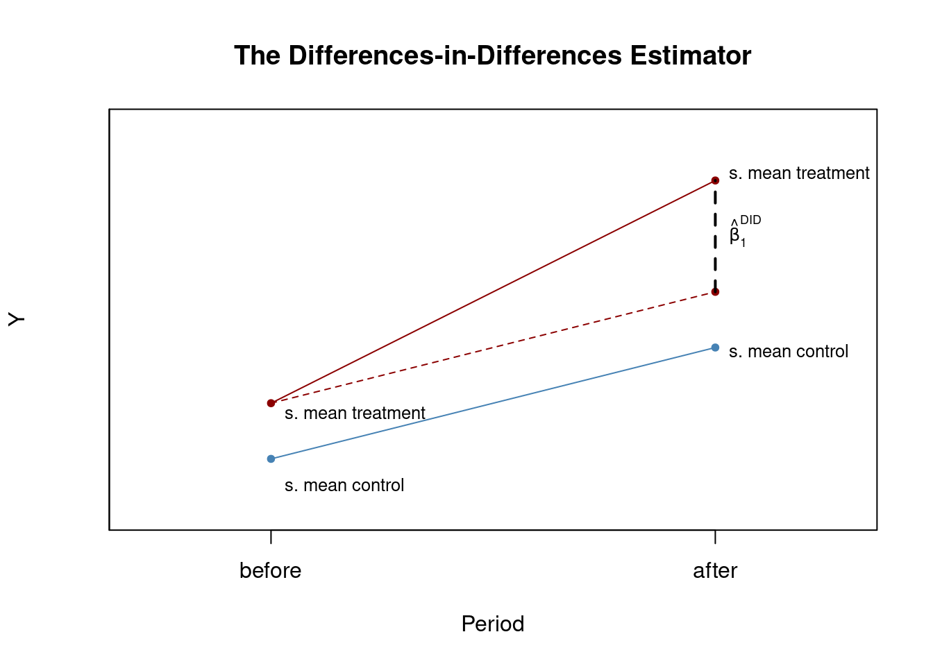
\widehat \beta_1^{\text{DID}} is the OLS estimator of \beta_1 in
\Delta Y_i = \beta_0 + \beta_1 X_i + u_i \tag{6.7}
where \Delta Y_i is the difference in pre- and post-treatment outcomes of individual i and X_i is the treatment indicator of interest.
If we add regressors measuring pre-treatment characteristics we have
\Delta Y_i = \beta_0 + \beta_1 X_i + \beta_2 W_{1i} + \cdots + \beta_{1+r} W_{ri} + u_i, \tag{6.8}
which is the difference-in-differences estimator with additional regressors.
Let’s simulate pre- and post-treatment data in R
# set sample size
n <- 200

# define treatment effect
TEffect <- 4

# generate treatment dummy
TDummy <- c(rep(0, n/2), rep(1, n/2))

# simulate pre- and post-treatment values of the dependent variable
y_pre <- 7 + rnorm(n)
y_pre[1:n/2] <- y_pre[1:n/2] - 1
y_post <- 7 + 2 + TEffect * TDummy + rnorm(n)
y_post[1:n/2] <- y_post[1:n/2] - 1
Now we plot the data. The jitter() function adds a bit of randomness to the horizontal positions of points, reducing overlap. Additionally, the alpha() function from the package scales lets you control how transparent the colors are in your plots.
library(scales)

pre <- rep(0, length(y_pre[TDummy==0]))
post <- rep(1, length(y_pre[TDummy==0]))

# plot control group in t=1
plot(jitter(pre, 0.6), y_pre[TDummy == 0],
     ylim = c(0, 16), col = alpha("steelblue", 0.3),
     pch = 20, xlim = c(-0.5, 1.5),
     ylab = "Y", xlab = "Period",
     xaxt = "n", main = "Artificial Data for DID Estimation")

axis(1, at = c(0, 1), labels = c("before", "after"))

# add treatment group in t=1
points(jitter(pre, 0.6), y_pre[TDummy == 1],
       col = alpha("darkred", 0.3), pch = 20)

# add control group in t=2
points(jitter(post, 0.6), y_post[TDummy == 0],
       col = alpha("steelblue", 0.5), pch = 20)

# add treatment group in t=2
points(jitter(post, 0.6), y_post[TDummy == 1],
       col = alpha("darkred", 0.5), pch = 20)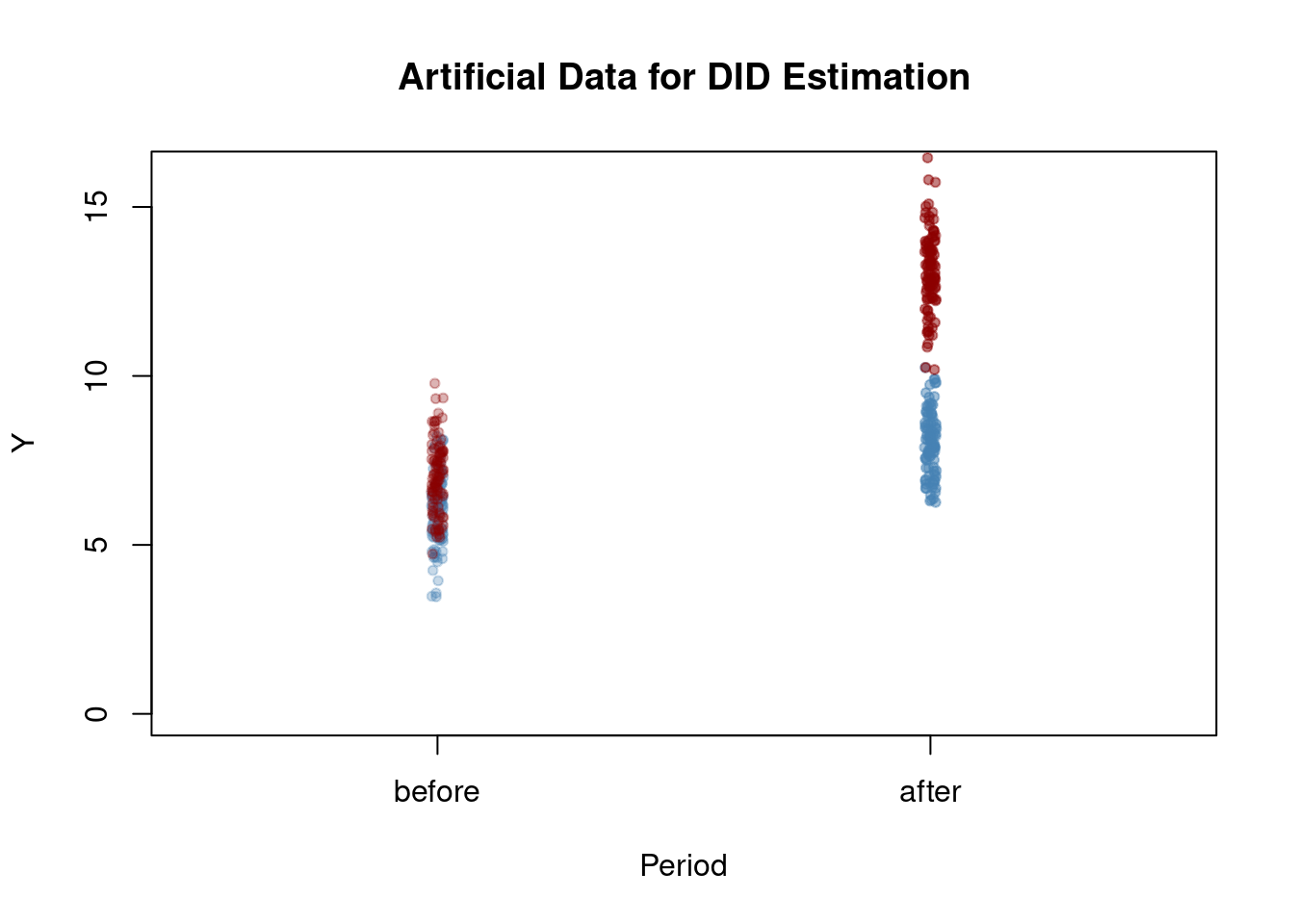
We observe higher average values for both groups after treatment, with a more pronounced increase observed in the treatment group. By employing the Differences-in-Differences (DID) method, we can assess the extent to which this disparity can be attributed to the treatment itself.
# compute the DID estimator for the treatment effect 'by hand'
mean(y_post[TDummy == 1]) - mean(y_pre[TDummy == 1]) -
(mean(y_post[TDummy == 0]) - mean(y_pre[TDummy == 0]))
[1] 4.044315The reported estimate is close to 4, the treatment effect value we previously selected for TEffect.
We can also obtain the DID estimator by performing OLS estimation of the simple linar model (6.7).
Call:
lm(formula = I(y_post - y_pre) ~ TDummy)

Coefficients:
(Intercept)       TDummy
      2.029        4.044
Lastly, we could alternatively compute the treatment effect by estimating \beta_{TE} in
Y_i = \beta_0 + \beta_1 D_i + \beta_2 Period_i + \beta_{TE}(Period_i \times D_i) + \epsilon_i, \tag{6.9} where D_i is the binary treatment indicator, Period a binary indicator for the after-treatment period and Period_i \times D_i is the interaction term of both.
# prepare data for DID regression using the interaction term
d <- data.frame("Y" = c(y_pre,y_post),
                "Treatment" = TDummy,
                "Period" = c(rep("1", n), rep("2", n)))

# estimate the model
lm(Y ~ Treatment * Period, data = d)
Call:
lm(formula = Y ~ Treatment * Period, data = d)

Coefficients:
      (Intercept)          Treatment            Period2  Treatment:Period2
            5.994              1.030              2.029              4.044
As we can see, the estimated coefficient on the interaction term is again the same DID estimate we computed before.
7.2 Regression Discontinuity Estimators
7.2.1 Sharp Regression Discontinuity
Let’s consider the model
Y_i = \beta_0 + \beta_1 X_1 + \beta_2 W_i + u_i \tag{6.10}
and let
X_i = \begin{cases} 1, & \text{if } W_i \geq c \\ 0, & \text{if } W_i < c, \end{cases}
so that the treatment receipt represented by X_i depends on a certain threshold c of a continuous variable W_i, known as the running variable.
We call (6.10)) a sharp regression discontinuity design because the treatment assignment is deterministic and continuous at the threshold: all observations with W_i \geq c are treated and those with W_i < c do not receive treatment.
The idea of regression discontinuity design is to use observations with a W_i close to c for the estimation of \beta_1, which is the average treatment effect for individuals with W_i=c, and is assumed to be a good approximation to the treatment effect in the population.
We will now estimate a linear SRDD, but first, we generate and plot some sample data
# load the package 'rddtools'
library(rddtools)

# construct rdd_data
data <- rdd_data(y, W, cutpoint = 0)

# plot the sample data
plot(data,
     col = "steelblue",
     cex = 0.35,
     xlab = "W",
     ylab = "Y")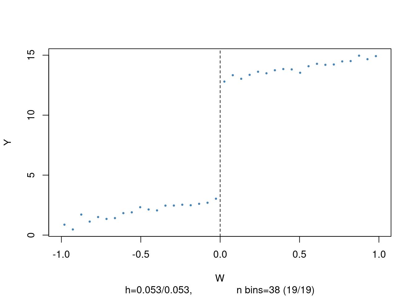
The dots in the plot represent bin averages of the outcome variable.
To estimate the treatment effect using model (6.10) on our generated data we can use rdd_reg_lm() from the rddtools package. By setting slope ="same" we ensure that the slopes of the regression function stay consistent on both sides of the threshold W=0.
# estimate the sharp RDD model
rdd_mod <- rdd_reg_lm(rdd_object = data,
                      slope = "same")
summary(rdd_mod)
Call:
lm(formula = y ~ ., data = dat_step1, weights = weights)

Residuals:
    Min      1Q  Median      3Q     Max
-3.4378 -0.7030 -0.0002  0.6786  3.1992

Coefficients:
            Estimate Std. Error t value Pr(>|t|)
(Intercept)   2.9944     0.0719   41.65   <2e-16 ***
D             9.9184     0.1304   76.05   <2e-16 ***
x             2.0487     0.1142   17.94   <2e-16 ***
---
Signif. codes:  0 '***' 0.001 '**' 0.01 '*' 0.05 '.' 0.1 ' ' 1

Residual standard error: 1.022 on 997 degrees of freedom
Multiple R-squared:  0.9719,    Adjusted R-squared:  0.9719
F-statistic: 1.726e+04 on 2 and 997 DF,  p-value: < 2.2e-16
The estimated coefficient on D represents the estimated treatment effect, which is very close to 10, the treatment effect we chose when generating the simulated data.
Let’s now visualize the result by plotting the estimated sharp RDD model
# plot the RDD model along with binned observations
plot(rdd_mod,
     cex = 0.35,
     col = "steelblue",
     xlab = "W",
     ylab = "Y")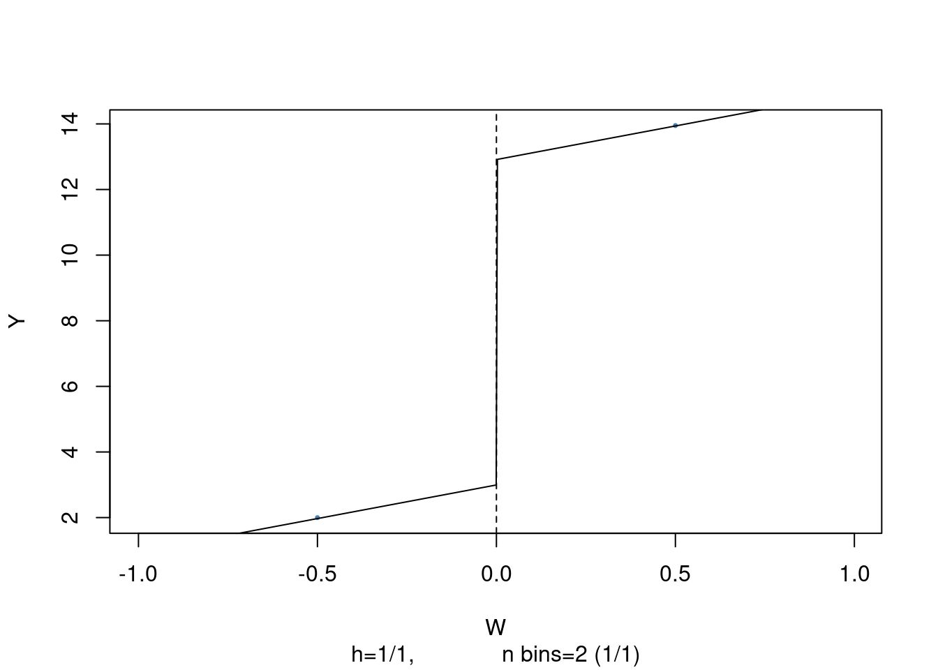
7.2.2 Fuzzy Regression Discontinuity
In the traditional setup, we assumed that crossing a threshold automatically leads to treatment, allowing us to see the jump in population regression functions at that point as the treatment’s effect.
However, when crossing the threshold doesn’t guarantee treatment (e.g. when other factors also influence who gets treated) we can’t rely on this assumption. Instead, we can view the threshold as a point where the likelihood of getting treated suddenly increases.
This increase might happen because of hidden factors affecting the chance of getting treated. So, the treatment variable X_i in the equation becomes correlated to the error term u_i, making it harder to accurately estimate the treatment’s effect.
In such cases, a fuzzy regression discontinuity design, which uses an instrumental variable (IV) approach, might help. We can use a binary variable Z_i to indicate whether the threshold is crossed or not.
Z_i = \begin{cases} 1, & \text{if } W_i \geq c \\ 0, & \text{if } W_i < c, \end{cases}
We assume that Z_i relates to Y_i only through the treatment indicator X_i, so Z_i and u_i are uncorrelated but Z_i influences the receipt of the treatment, so it is correlated with X_i. Therefore, Z_i is a valid instrument for X_i and we can estimate (6.10) via TSLS.
Let’s now assume that observations with a value of W_i below 0 do not receive the treatment and those with W_i \geq 0 have a 80\% probability of being treated. The treatment effect leads to an increase in the dependent variable of 2 points.
library(MASS)

# generate sample data
mu <- c(0, 0)
sigma <- matrix(c(1, 0.7, 0.7, 1), ncol = 2)

set.seed(1234)
d <- as.data.frame(mvrnorm(2000, mu, sigma))
colnames(d) <- c("W", "Y")

# introduce fuzziness
d$treatProb <- ifelse(d$W < 0, 0, 0.8)

fuzz <- sapply(X = d$treatProb, FUN = function(x) rbinom(1, 1, prob = x))

# treatment effect
d$Y <- d$Y + fuzz * 2
We now plot the observations using blue for non-treated and red for treated units.
# generate a colored plot of treatment and control group
plot(d$W, d$Y,
     col = c("steelblue", "darkred")[factor(fuzz)],
     pch= 20,
     cex = 0.5,
     xlim = c(-3, 3),
     ylim = c(-3.5, 5),
     xlab = "W",
     ylab = "Y")

# add a dashed vertical line at cutoff
abline(v = 0, lty = 2)
#add legend
legend("topleft",pch=20,col=c("steelblue","darkred"),
       legend=c("Do not receive treatment","Receive treatment"))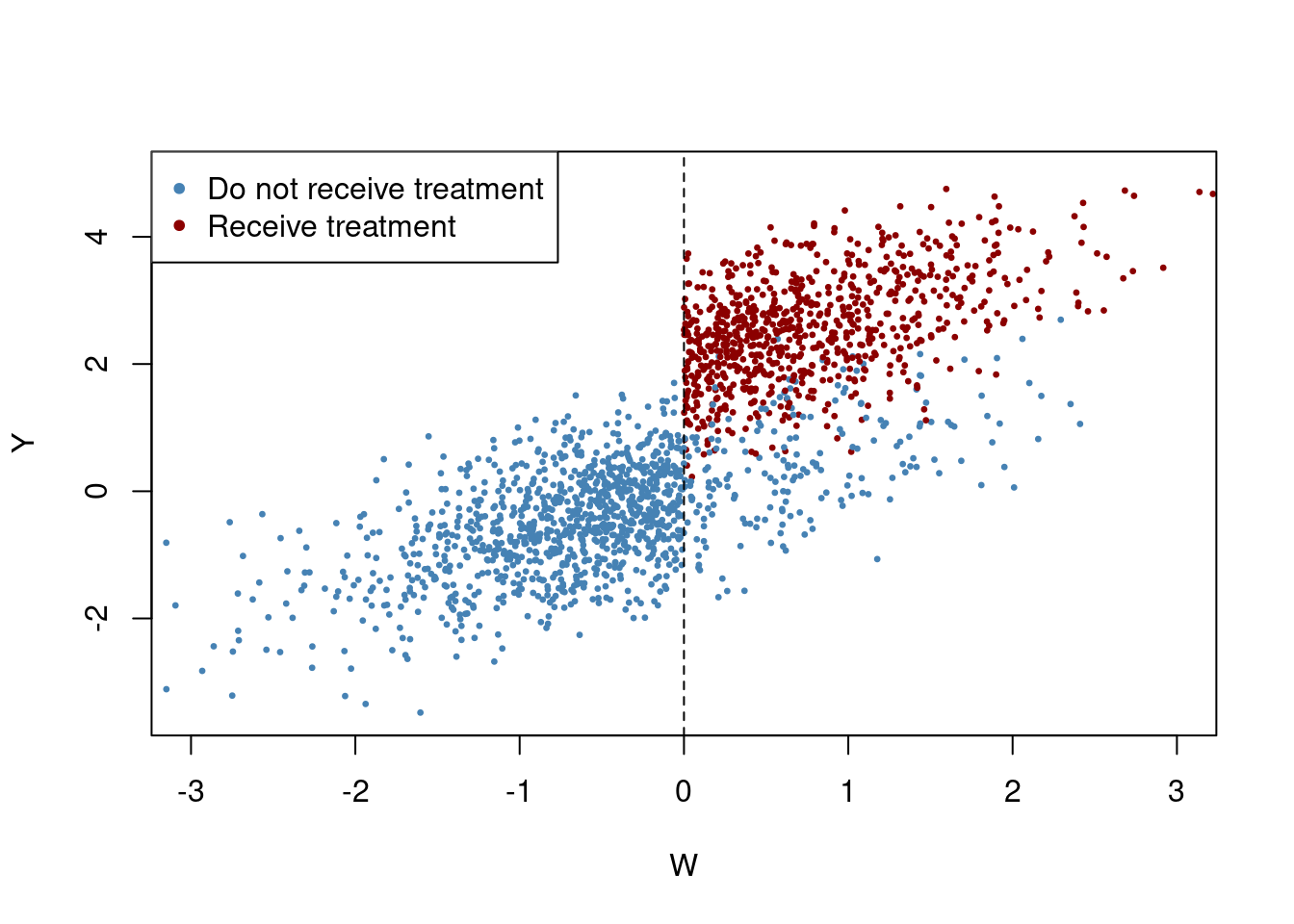
As we can observe, the receipt of treatment is no longer a deterministic function of the running variable W, since some observations with W \geq 0 did not receive the treatment.
We can estimate a FRDD by setting treatProb as the assignment variable z in rdd_data(). The function rdd_reg_lm() applies a TSLS procedure:
In the first stage regression, treatment is predicted using W_i and the cutoff dummy Z_i, the instrumental variable.
Using the second stage, where the outcome Y is regressed on the fitted values and the running variable W, we obtain a consistent estimate of the treatment effect.
# estimate the Fuzzy RDD
data <- rdd_data(d$Y, d$W,
                 cutpoint = 0,
                 z = d$treatProb)

frdd_mod <- rdd_reg_lm(rdd_object = data,
                       slope = "same")
frdd_mod
### RDD regression: parametric ###
Polynomial order: 1
Slopes: same
Number of obs: 2000 (left: 999, right: 1001)
Coefficient:
Estimate Std. Error t value Pr(>|t|)
D 1.981297 0.084696 23.393 < 2.2e-16 ***
---
Signif. codes: 0 '***' 0.001 '**' 0.01 '*' 0.05 '.' 0.1 ' ' 1The estimated treatment effect is very close to 2, which is the real treatment effect. We can now plot the estimated regression function and the binned data.
# plot estimated FRDD function
plot(frdd_mod,
     cex = 0.5,
     lwd = 0.4,
     xlim = c(-4, 4),
     ylim = c(-3.5, 5),
     xlab = "W",
     ylab = "Y")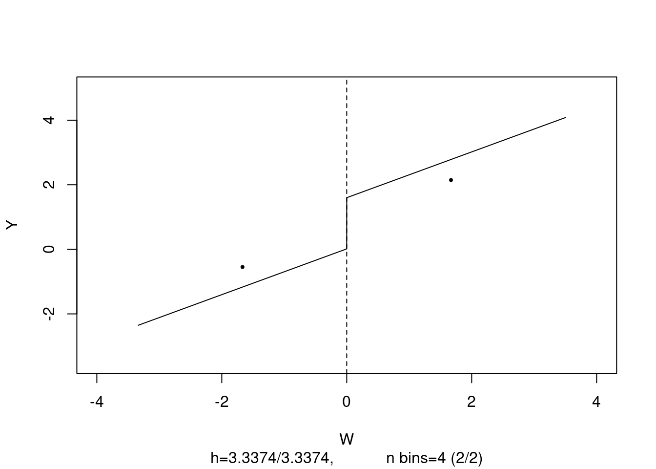
What if we opted for a Sharp Regression Discontinuity Design (SRDD), disregarding the fact that treatment isn’t solely determined by the cutoff in W? We can explore the potential outcomes by estimating an SRDD using the data we simulated earlier.
# estimate SRDD
data <- rdd_data(d$Y,
                 d$W,
                 cutpoint = 0)

srdd_mod <- rdd_reg_lm(rdd_object = data,
                       slope = "same")
srdd_mod
### RDD regression: parametric ###
Polynomial order: 1
Slopes: same
Number of obs: 2000 (left: 999, right: 1001)
Coefficient:
Estimate Std. Error t value Pr(>|t|)
D 1.585038 0.067756 23.393 < 2.2e-16 ***
---
Signif. codes: 0 '***' 0.001 '**' 0.01 '*' 0.05 '.' 0.1 ' ' 1The estimate using SRDD indicates a significant downward bias. This method is not reliable for determining the true causal effect, meaning that increasing the sample size wouldn’t fix the bias issue.
7.3 Discussion
In the book by Stock and Watson the potential problems with quasi-experiments are discussed, focusing on threats to internal and external validity.
Internal validity threats include failure of randomization and failure to follow the treatment protocol, which can lead to biased estimators. They highlight the importance of testing for systematic differences between treatment and control groups to assess the reliability of quasi-experiments.
Additionally, they address attrition and instrument validity, emphasizing the need for careful consideration of instrument relevance and exogeneity.
External validity threats in quasi-experiments are similar to those in conventional regression studies, with special events creating challenges for generalizability.
Lastly, Stock and Watson discuss estimating causal effects in heterogeneous populations, where individuals may have different treatment effects; OLS estimators are consistent for the average causal effect, but instrumental variables (IV) estimators may estimate a weighted average of individual effects, known as the local average treatment effect (LATE), highlighting the importance of understanding how individuals’ treatment decisions affect estimation.