13 Econometric Analysis of Time Series
13.1 ARIMA models
Let \color{blue}{y_t = Y_t - \mu} with \mu = E(Y_t) a demeaned time series for t = 1, \ldots, T
Autoregressive model of order p:
\begin{align*} \text{AR}(p) \quad &y_t = \color{blue}{\theta_1 y_{t-1} + \cdots + \theta_p y_{t-p}} + \varepsilon_t \\ &\theta(L) y_t = \varepsilon_t \end{align*}
where \color{red}{\theta(L) = 1 - \theta_1 L - \cdots - \theta_p L^p}
Moving-Average model of order q:
\begin{align*} \text{MA}(q) \quad y_t &= \varepsilon_t \color{blue}{+ \alpha_1 \varepsilon_{t-1} + \cdots + \alpha_q \varepsilon_{t-q}} \\ y_t &= \alpha(L) \varepsilon_t \end{align*}
where \color{red}{\alpha(L) = 1 + \alpha_1 L + \cdots + \alpha_q L^q}
ARMA (p,q) model:
\theta(L) y_t = \alpha(L) \varepsilon_t
Autoregressive representation of a ARMA(p, q):
\color{blue}{\frac{\theta(L)}{\alpha(L)}} \color{black}{ y_t = \tilde\theta(L) y_t = \varepsilon_t}
\tilde\theta(L) can be determined by comparing coefficients from
\alpha(L) \tilde\theta(L) = \theta(L)
Any ARMA(p, q) model can be approximated by a AR(p) model choosing \tilde p large enough
A time series is stationary if \theta(L) is invertible, i.e., if it can be factorized as
\theta(L) = (1 - \phi_1 L)(1 - \phi_2 L) \cdots (1 - \phi_p L)
such that it holds that |\phi_i| < 1 for all 1 = i, \ldots, p.
Alternatively, \theta(L) is invertible if the p roots z_1, \ldots, z_p of the characteristic equation
\theta(z) = 0
are all outside the unit circle of the complex plane. For real root we have z_i = 1/\phi_i.
13.2 Unit roots
An important special case results if \phi_1 = 1, that is,
\theta(L) y_t = (1 - L)(1 - \phi_2 L) \cdot (1 - \phi_p L) = \theta^*(L) \Delta y_t = \varepsilon_t
where all other roots are outside the unit circle, i.e., \Delta y_t is stationary.
if p = 1, then y_t is white noise (serially uncorrelated) and y_t is a random walk with
y_t = y_{t-1} + \varepsilon_t = \varepsilon_t + \varepsilon_{t-1} + \cdots + \varepsilon_1 + y_0 such that \text{var}(y_t) = \text{var}(y_0) + t\sigma^2
a time series is (weakly) stationary if
E(y_t) = 0 \quad \text{ and } \quad var(y_t) = \sigma^2_y \quad \text{ for all } t
\Rightarrow a random walk with \theta(L) = 1-L is nonstationary
Unit root test
\phi_1 = 1 implies \theta(1) = 0 (one root is on the unit circle)
\begin{align*} y_t &= \theta y_{t-1} + \varepsilon_t \\ \Leftrightarrow \color{blue}{\Delta y_t} &= \color{blue}{\underbrace{(\theta - 1)}_{\pi} y_{t-1} + \varepsilon_t} \end{align*}
can be tested by using the t-statistic for \pi = 0 (Dickey-Fuller statistic):
\text{DF-t} = \frac{\widehat{\theta} - 1}{\text{se}(\hat{\theta})} = \frac{\hat{\pi}}{\text{se}(\hat{\pi})}
Problem: t-statistic is NOT t-distributed
Extension to unknown mean and trend:
\begin{align*} \Delta Y_t &= \color{red}{\delta \, + } \, \color{black}{ \pi y_{t-1} + \varepsilon_t} \\ \text{or} \quad \Delta Y_t &= \color{red}{\delta + \gamma t \, +} \, \color{black}{\pi y_{t-1} + \varepsilon_t} \end{align*}
Different critical values for models (i) no constant (ii) with a constant and (iii) with a time trend.
Include a trend if the series seem to evolve around a (linear) time trend
Extension to AR(p) models:
\begin{align*} y_t &= \color{blue}{\delta \, [+ \gamma t] \, +} \, \color{black}{\theta_1 y_{t-1} + \theta_2 y_{t-2} + \cdots + \theta_p y_{t-p} + \varepsilon_t} \\ \Leftrightarrow \Delta y_t &= \color{blue}{\delta \, [+ \gamma t] \, +} \, \color{black}{\pi y_{t-1} + c_1 \Delta y_{t-1} + \cdots + c_{p-1} \Delta y_{t-p} + \varepsilon_t} \end{align*}
critical values do NOT depend on the lag-order p
A series is called “integrated of order d” or \color{red}{y_t \sim I(d)} if \Delta^d y_t is stationary but \Delta^{d-1} is nonstationary
\Rightarrow DF tests are used to determine d empirically
13.3 Cointegration
Assume:
Y_t \sim I(1) \quad \text{and} \quad X_t \sim I(1)
\Rightarrow In general Y_t - \beta X_t is also I(1)
Spurious regression: If y_t and x_t are independent random walks:
- t-values are often significant
- large R^2
- Low Durbin-Watson statistic
Common trend model (“cointegration”)
\begin{align*} &X_t = r_t + u_{1t} \, \color{blue}{\sim I(1)} \\ &Y_t = \beta r_t + u_{2t} \, \color{blue}{\sim I(1)} \\ &\color{blue}{Y_t - \beta X_t \,} \color{black}{ = u_{2t} - \beta u_{1t} = u_t} \, \color{red}{ \sim I(0)} \end{align*}
where \color{red}{r_t \sim I(1)} (stochastic trend) and u_t is stationary
Estimation and testing
Properties of OLS in cointegrating regressions:
\widehat\beta - \beta is O_p(T^{-1}) (“super-consistent”)
robust against endogenous X_t
Efficient only if (i) X_i is exogenous (ii) u_t is serially uncorrelated
t statistics are generally invalid
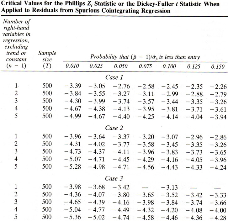
Test for cointegration:
Step: ADF test of Y_t and X_t
Step: ADF test of the residuals e_t= Y_t - X_t \hat\beta
Critical values depend also on K
Engle-Granger two-step approach
Error correction representation:
Y_t = \delta + \alpha Y_{t-1} + \beta_1 X_{t-1} + \beta_2 X_{t-2} + u_t
can be rewritten as
\begin{align*} \Delta Y_t &= \delta + \phi_1 \Delta X_{t-1} + \gamma \color{blue}{(Y_{t-1} - \beta X_{t-1})} \color{black}{+ u_t} \\ & \\ \text{where} \quad &\phi_1 = -\beta_2, \quad \gamma = \alpha - 1 < 0, \quad \text{and} \quad \beta = (\beta_1 + \beta_2) / (1 - \alpha) \end{align*}
\color{blue}{(Y_{t-1} - \beta X_{t-1}) \sim I(0)} is called the error correction term
replace \beta by \hat\beta (Engle/Granger 2-step estimator)
Coefficients attached to stationary variables have the usual asymptotic distributions (t-statistics yield valid tests)