10 Limited Dependent Variables
Binary choice models
Choice based on Utility
\begin{align*} U_{i0} &= x'_i \gamma_0 + \epsilon_{i0} \\ U_{i1} &= x'_i \gamma_1 + \epsilon_{i1} \end{align*}
where
\begin{align*} U_{ij} &: \text{utility due to the choice of j} \\ x_i &: \text{variables characterizing the individual i} \end{align*}
Decision rule:
\begin{align*} y^*_i &= U_{i1} - U_{i0} = \begin{cases} \color{red}{> 0} & \Rightarrow \text{ choose 1} \\ \leq 0 & \Rightarrow \text{ choose 0} \end{cases} \\ y^*_i &= x'_i \color{blue}{(\gamma_1 - \gamma_0)} \color{black}{+ \epsilon_{i1} - \epsilon_{i0}} \\ &= x'_i \color{blue}{\beta} \color{black}{+ \epsilon_i} \end{align*}
where \varepsilon_i = \epsilon_{i1} - \epsilon_{i0}
10.1 Linear probability model
y^*_i in the binary choice model is typically not observed. What we observe is:
y_i = \begin{cases} 1 & \text{for } y^*_i > 0, \\ 0 & \text{for } y^*_i \leq 0. \end{cases} Assuming that the probability function is linear we have
\begin{align*} E(y_i | x_i) &= \color{blue}{P(y_i = 1 | x_i)} \color{black}{\cdot 1 + } \color{red}{P(y_i = 0 | x_i)} \color{black}{\cdot 0} \\ &= x'_i \beta \end{align*}
In this case we can estimate the linear regression:
y_i = x'_i \beta + u_i A linear probability function is pretty unrealistic and implies that \varepsilon_i is uniformly distributed (see below)
The errors u_i are heteroskedastic (variance depends on x_i). Robust standard errors are required.
10.2 Probit/Logit models
Consider the binary choice model with
\begin{align*} P(y_i = 1) &= P(\varepsilon_i > -x'_i \beta) \\ &= 1 - F(-x'_i \beta) \end{align*}
where F(\cdot) denotes the distribution function of \varepsilon_i
It follows that
\begin{align*} E(y_i | x_i) &= 1 - F(-x'_i \beta)\\ &= F(x'_i \beta) \text{ if the distribution is symmetric} \end{align*}
Nonlinear regression model:
\begin{align*} y_i &= \color{blue}{E(y_i | x_i)} \color{black}{+ u_i} \\ &= \color{red}{F(x'_i \beta)} \color{black}{+ u_i \quad \text{for symmetric distributions}} \end{align*}
error is (centered) binomially distributed with p_i = F(x'_i \beta)
estimation with Maximum Likelihood (similar to nonlinear regression)
Popular distributions:
\begin{align*} F &\sim \color{red}{\text{normal} \color{black}{\text{ distribution}}} \\ &\sim \color{blue}{\text{logistic} \color{black}{\text{ distribution}}} \end{align*}
Choice of the Distribution:
- Usually no information about the distribution
- Referring to the central limit theorem
- Practical reasons
- Specification tests
- Nonparametric estimation
Normal distribution (“Probit”) F \equiv \Phi(z) = \int_{-\infty}^{z} \frac{1}{\sqrt{2\pi}} e^{-u^2 / 2} \, du Logistic distribution (“Logit”)
F \equiv L(z) = \frac{1}{1 + e^{-z}}

Both distributions are symmetric:
1 -F(-z) = F(z) and therefore: y_i = \color{blue}{F (x'_i\beta)} \color{black}{+ v_i}
Both distributions are very similar \Phi(z) \approx L\left(\frac{\pi}{\sqrt{3}}z\right)
Marginal probability effect
partial effect of x_i on y_i
MPE_i = \frac{\partial F(x'_i \beta)}{\partial x_i} = \color{red}{\phi(x'_i \beta)} \color{black}{ \beta} \Rightarrow effect depends on the level of x_i
Maximum likelihood (ML) estimator
log-likelihood function for a symmetric distribution:
\log L(\beta) = \sum_{i=1}^{N} \color{blue}{y_i} \color{red}{ \log F(x'_i \beta)}\color{black}{ + } \color{blue}{(1 - y_i)} \color{red}{\log[1 - F(x'_i \beta)]}
Differentiation with respect to \beta yields the first order condition:
s(\widehat{\beta}) = \sum_{i=1}^{N} \frac{e_i f(x'_i \widehat{\beta})}{F(x'_i \widehat{\beta})(1 - F(x'_i \widehat{\beta}))} x_i = 0
where e_i = y_i - F(x'_i \widehat{\beta})
Nonlinear system of K equations: Iterative algorithm
Estimator is equivalent to nonlinear LS with heteroskedasticn errors
Goodness of fit
(i) McFadden R^2:
\text{MF-}R^2 = 1 - \frac{\log L(\widehat{\beta})}{\log L(\beta = 0)}
(ii) forecasting y_i: Let
\widehat{y}_i = \begin{cases} 1 & \text{if } \color{blue}{F(x'_i \widehat{\beta}) > 0.5} \color{black}{\text{ or } x'_i \widehat{\beta} > 0,} \\ 0 & \text{otherwise} \end{cases} frequency of wrong forecasts:
\frac{n_{01} + n_{10}}{n} = \frac{\sum_{i=1}^{n} (y_i - \widehat{y_i})^2}{n}
\Rightarrow R^2 based on the number of wrong forecasts
10.3 Classification
Let F_i denote the estimated probability for y_i = 1. The optimal assignment to the unknown alternatives {0, 1} is \widehat{y_i} = 1 if F_i > 0.5.
This classification rule works poorly if F_i is small. Assume that x_i \sim \text{U}[0, 1] and
y^*_i = -2 +2x +u_i
then the probability for y_i = 1 is 0.2, but in the sample, no unit value is predicted!
One may calibrate the threshold to reduce the classification error such that
\sum_{i=1}^{n} 1(\widehat{F_i} > \tau) = \sum_{i=1}^{n} y_i
\Rightarrow match the unconditional probabilities.
Trade-off between the two types of misclassification
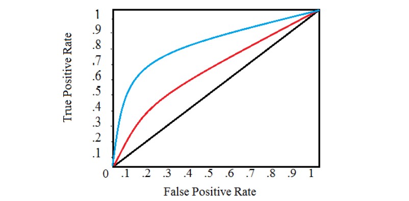
Useful tool: ROC curve (true positive vs. false positive) If \tau is decreased \rightarrow more ONEs. These can be correct and false detections.
A classification blue is uniformly better than red if ROC is always above ROC
\Rightarrow maximize the area below the ROC curve
The target of the Probit/Logit estimator is P(y_i = 1) = F(x'_i\beta). The optimal estimator of the probability coincides with the efficient estimator of \beta.
The classification problem seeks an “optimal” estimator for y_i based on the indicator function \widehat{y_i} by minimizing some combination of the (error rates):
\begin{align*} \text{False Positive} &= \sum_{i} y_i (1 - \widehat{y_i}) / \sum_{i} y_i \quad\text{and} \\ \text{False Negative} &= \sum_{i} (1 - y_i) \widehat{y_i} / \sum_{i} (1 - y_i) \end{align*}
Note that F(x'_i \beta) > \tau is equivalent to x'_i \beta > \tau^* with \tau^* = F^{-1}(\tau). \Rightarrow distribution not relevant for classification
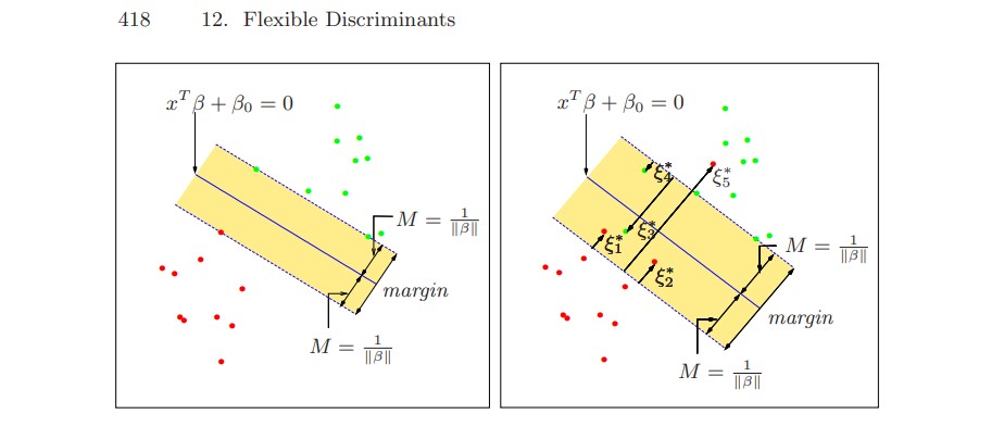
Support vector classifier: Maximize M subject to:
\begin{align*} &(2y_i - 1)(x'_i \beta) \geq M(1 - \xi_i) \\ &\xi_i > 0, \quad \sum \xi_i \leq C \\ &\beta' \beta = 1 \end{align*}
10.4 Sample selection model
\begin{align*} \color{blue}{\text{Regression model:}} \quad &y_i = x'_{1i}\beta_1 + u_{1i} \quad \color{blue}{\text{if } h_i = 1} \\ \color{red}{\text{Selection rule:}} \quad &h^*_i = x'_{2i}\beta_2 + u_{2i} \quad \text{with } E(u^2_{2i}) = 1 \\ \\ &h_i = \begin{cases} 1 & \text{if } h^*_i > 0 \quad \color{red}{\text{observed}} \\ 0 & \text{otherwise} \quad \color{red}{\text{not observed}} \end{cases} \end{align*}
Equivalent to the Tobit model if:
x_{1i} = x_{2i}, \quad \beta_1 / \sigma = \beta_2, \quad u_{1i} / \sigma = u_{2i}
truncated joint density
E(y_i | \color{red}{y_i \text{ observed}}\color{black}{) = x'_{1i}\beta +} \color{red}{\varrho\sigma} \color{black}{\lambda_i}
where \varrho = E(u_{1i}u_{2i})/\sigma and
\lambda_i = \frac{\phi(x'_{2i}\beta_2)}{\Phi(x'_{2i}\beta_2)}
Heckman estimator
First step: Probit estimator
\tilde{y}^*_i = x'_i \tilde{\beta} + u_i
where \tilde{\beta} = \beta / \sigma and
y_i = \begin{cases} 1 & \text{if } \tilde{y}^*_i > 0 \\ 0 & \text{otherwise} \end{cases}
Second step: augmented regression:
\lambda_i = \frac{\phi(x'_i \tilde{\beta})}{\Phi(x'_i \tilde{\beta})}
and
y_i | y^*_i > 0 = x'_i \beta + \sigma \color{red}{\hat{\lambda}_i} \color{black}{ + \nu_i}
Standard errors are biased
ML estimator is available