11 Causal Inference
11.1 Experiments and Treatment Effects
Causal effects as measured in (double blind) clinical trials
Separation into two groups a) with treatment b) without treatment (placebo)
Quasi-experiment: because of external events the treatment of some individual occurs as if it is random
Let Y (X) denote the (potential) outcome variable, depending on the binary treatment indicator X_i:
\begin{align*} Y_i | X_i &= 1: \text{ outcome with treatment} \\ Y_i | X_i &= 0: \text{ outcome without treatment} \end{align*}
Average causal effect: E(Y_i | X_i = 1) - E(Y_i | X_i = 0)
Problem: only one of the two possible outcomes is observed the other is counterfactual
Regression based analysis of treatment effects
- Difference estimator
Y_i = \beta_0 + \color{red}{\beta_1}\color{black}{X_i + u_i}
The OLS estimator is equivalent to
\widehat{\beta_1} = \frac{1}{n_1} \sum_{i: X_i = 1} Y_i - \frac{1}{n_0} \sum_{i: X_i = 0} Y_i
with n_1 = \sum{X_i} (number of treated units) and n_0 = n ??? n_1
The estimator is unbiased for random assignment: \color{blue}{E(u_i | X_i = 1) = E(u_i) = 0}
Regression with pre-treatment characteristics W_i
\begin{align*} y_i &= \beta_0 + \color{red}{\beta_1} \color{black}{ X_i + \beta_2 W_{1i} + \cdots + \beta_{r+1} W_{ri} + u_i} \\ &= \beta_0 + \color{red}{\beta_1} \color{black}{X_i + \beta'_2 \mathbf{w}_i + u_i \quad \text{where } \mathbf{w}_i = (W_{1i}, \ldots, W_{ri})'} \end{align*}
E(u_i | X_i = 1, \color{blue}{w_i} \color{black}{) = E(u_i |} \color{blue}{ w_i} \color{black}{) = 0}
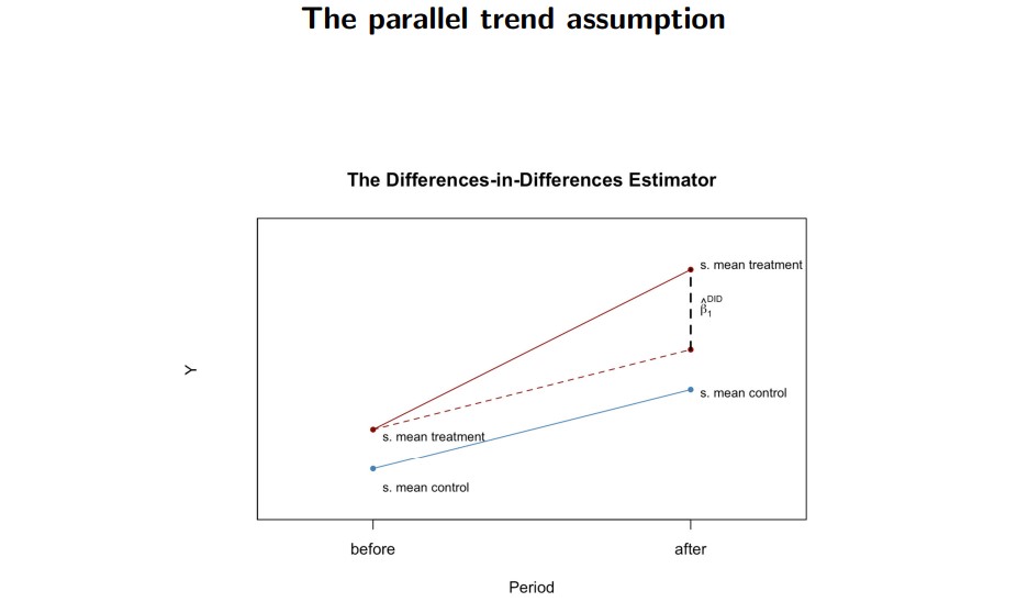
11.2 Difference-in-Difference (DiD) estimation
“Before and After” comparisons
Example: happiness before and after marriage
estimation by entity-demeaning is equivalent to:
Y_{it} = \beta_0 + \underbrace{ \color{red}{\beta_1} \color{black}{(t \cdot X_i)}}_{\text{treatment effect}} + \beta_2 X_i + \beta_3 t + u_{it}
where X_i is the treatment dummy and t \in \{0, 1\} is the period dummy
How does the Fatality Rate (FR) change after a change in the beer tax?
FR_{1988} - FR_{1982} = -0.072 \color{red}{-1.04} \color{black}{ (tax_{1988} ??? tax_{1982})} where the relevant t-statistic is -1.04/0.36 = 2.888 (significant)